Tartalomjegyzék

Isidori I., Example 4.1.4. Feedback linearization

Teljes Matlab script kiegészítő függvényekkel.

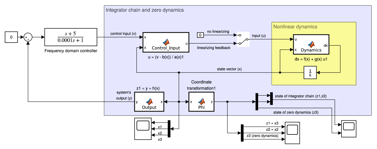
Coordinate transformation, feedback linearization and zero dynamics.

File: ccs_nonlin_Isidori_Ex414_feedbacklin.m
Directory: 4_gyujtemegy/11_CCS/_2_nonlin-pannon/2018
Author: Peter Polcz (ppolcz@gmail.com)

Created on 2018. July 29.

Prerequisites (1st Matlab practice)

Addition Mathematica calculations

Published Mathematica notebook: Integral_PDE_Public.pdf.

You can download the source notebook: Integral_PDE_Public.nb

Model description

syms t u v real
syms x1 x2 x3 real
syms z1 z2 z3 real

x = [x1 ; x2 ; x3];
z = [z1 ; z2 ; z3];

d = @(g) jacobian(g,x);
Lie = @(f,g) d(g)*f;
br = @(f,g) d(g)*f - d(f)*g;

f = [ -x1 ; x1*x2 ; x2 ];
g = [ exp(x2) ; 1 ; 0 ];
h = x3;

phi3 = 1 + x1 - exp(x2);

Phi = [
    h
    Lie(f,h)
    phi3
    ];
Phi_fh = matlabFunction(Phi, 'vars', {x});

% Compute equilibrium point
sol = struct2cell(solve(f,x));
xeq = [ sol{:} ]';
zeq = Phi_fh(xeq);

% Quick check: should be zero
% Lie(g,phi3)

\begin{align}\Phi(x) = \left(\begin{array}{c} x_{3}\\ x_{2}\\ x_{1}-{\mathrm{e}}^{x_{2}}+1 \end{array}\right)\end{align}

Quick check

\begin{align}L_g \phi_3(x) = 0\end{align}

$\phi_3(x)$ is given by Isidori, but anyone can check that this is indeed a solution for the PDE. This solution can also be computed by Mathematica.

Phi_inv = struct2cell(solve(z-Phi, x));
Phi_inv = [ Phi_inv{:} ]';
Phi_inv_fh = matlabFunction(Phi_inv, 'vars', {z});

Check if it is indeed the good inverse: $\Phi\big(Phi^{-1}(z)\big) = z$ and $\Phi^{-1}\big(\Phi(x)\big) = x$

simplify(Phi_fh(Phi_inv))
simplify(Phi_inv_fh(Phi))

Output:

ans =
 z1
 z2
 z3
ans =
 x1
 x2
 x3

\begin{align}\Phi^{-1}(z) = \left(\begin{array}{c} z_{3}+{\mathrm{e}}^{z_{2}}-1\\ z_{2}\\ z_{1} \end{array}\right)\end{align}

Coordinate transformation

b = Lie(f, Lie(f,h));
a = Lie(g, Lie(f,h));
q3 = Lie(f, Phi(3));

\begin{align}b(x) = x_{1}\,x_{2},~ a(x) = 1,~ q_3(x) = -x_{1}-x_{1}\,x_{2}\,{\mathrm{e}}^{x_{2}}\end{align}

b = subs(b, x, Phi_inv);
a = subs(a, x, Phi_inv);
q3 = subs(q3, x, Phi_inv);

\begin{align}b(z) = z_{2}\,\left(z_{3}+{\mathrm{e}}^{z_{2}}-1\right),~ a(z) = 1,~ q_3(z) = 1-{\mathrm{e}}^{z_{2}}-z_{2}\,{\mathrm{e}}^{z_{2}}\,\left(z_{3}+{\mathrm{e}}^{z_{2}}-1\right)-z_{3}\end{align}

dz = simplify([ z2 ; collect(b+a*u,u) ; q3 ]);

System dynamics in the new coordinates

\begin{align}\dot z = \left(\begin{array}{c} z_{2}\\ u+z_{2}\,\left(z_{3}+{\mathrm{e}}^{z_{2}}-1\right)\\ -\left(z_{2}\,{\mathrm{e}}^{z_{2}}+1\right)\,\left(z_{3}+{\mathrm{e}}^{z_{2}}-1\right) \end{array}\right)\end{align}

Linearizing feedback design

u_fdb = a \ (-b + v);

\begin{align}u = v-z_{2}\,\left(z_{3}+{\mathrm{e}}^{z_{2}}-1\right)\end{align}

Closed loop

dz_fdb = simplify(subs(dz, u, u_fdb));

\begin{align}\dot z = \left(\begin{array}{c} z_{2}\\ v\\ -\left(z_{2}\,{\mathrm{e}}^{z_{2}}+1\right)\,\left(z_{3}+{\mathrm{e}}^{z_{2}}-1\right) \end{array}\right)\end{align}

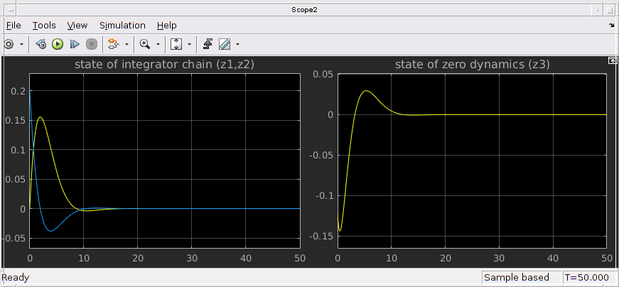
Zero dynamics

Zero_dynamics = simplify(subs(dz_fdb(3), [z ; v], [zeq ; 0]));

The zero dynamics is stable in the origin.

\begin{align}\dot z_3 = 0\end{align}

Linearized dynamics

Overall dynamics without the zero dynamics.

A = [
    0 1
    0 0
    ];

B = [
    0
    1
    ];

C = [ 1 0 ];

sys = ss(A,B,C,0);

s = tf('s');

H = tf(sys)

eps1 = 0.01;
eps2 = 0.01;

H_control = s^2/(eps1*s^2 + eps2*s + 1);

He = minreal(feedback(H*H_control,1))

[POLES, ZEROS] = pzmap(He)

Output:

H =
 
   1
  ---
  s^2
 
Continuous-time transfer function.


He =
 
       100
  -------------
  s^2 + s + 200
 
Continuous-time transfer function.

POLES =
  -0.5000 +14.1333i
  -0.5000 -14.1333i
ZEROS =
  0×1 empty double column vector

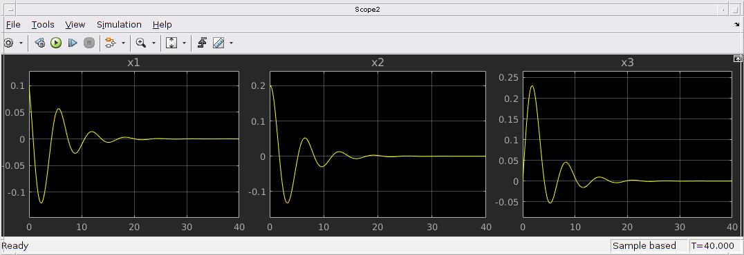
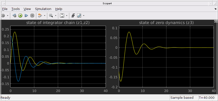
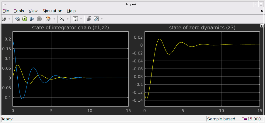
Frequency domain controller for the integrator chain

Transfer function of the feedback controller $H(s) = \frac{s + 5}{\alpha s + 1}$.

Download model here: Isidori_Example414_PID.slx

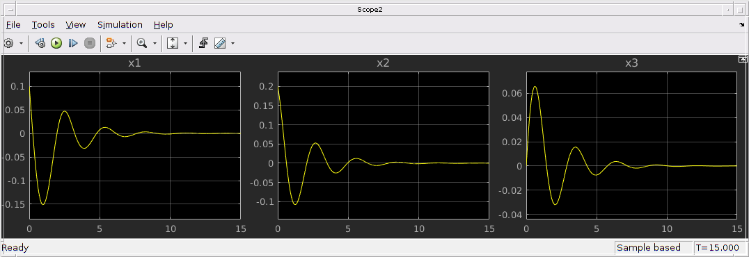
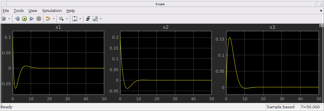
Pole placement controller

Download model here:

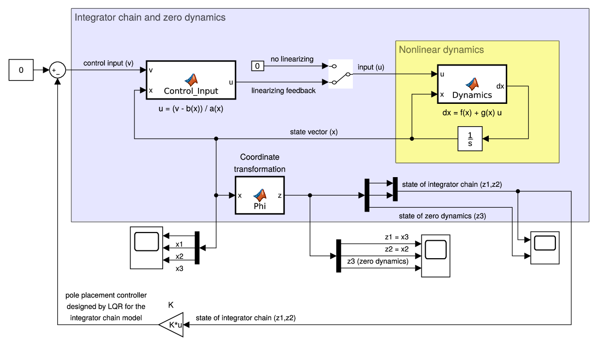
% State feedback gain designed by LQR
K = lqr(A,B,0.1*eye(2),1);

Pole placement controller with observer (just for fun)

Note that when a linearizing feedback is applied, we need to know the full state vector. But we can play a little bit, what if we forget the values of the state variables.

Download model here: Isidori_Example414_obs_state_feedback.slx

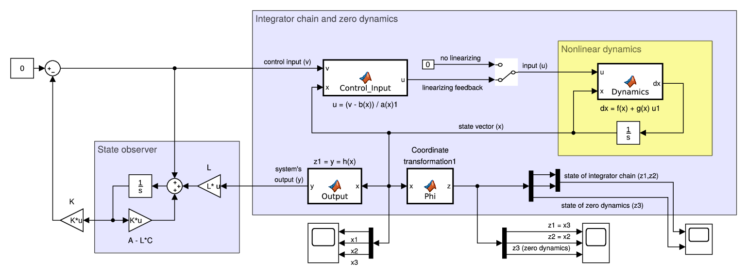
% Observer for integrator chain
L = place(A',C',[-2 -3])';

% State feedback gain designed by LQR
K = lqr(A,B,0.1*eye(2),1);

Published with MATLAB® R2017b, and sanitarized by BeautifulSoup (Python script using BSoup is written by Polcz).