Tartalomjegyzék

Frequency domain analysis

Teljes Matlab script kiegészítő függvényekkel.

File: minimum_phase_systems.m
Directory: 4_gyujtemegy/11_CCS/04_frequency_domain_analysis
Author: Peter Polcz (ppolcz@gmail.com)

Created on 2018. April 22.

Automatically generated stuff

Output:

 
┌ <a href="matlab:edit('/home/ppolcz/Repositories/Bitbucket/control-systems/4_gyujtemegy/11_CCS/04_frequency_domain_analysis/minimum_phase_systems.m')">minimum_phase_systems</a> called from <a href="matlab:opentoline('',115)">instrumentAndRun:115</a>
│   [  <strong>INFO </strong> ] Persistence for `minimum_phase_systems` reused (inherited) [run ID: 0622, 2018.04.22. Sunday, 20:14:36]
│   [  <strong>INFO </strong> ] Script `minimum_phase_systems` backed up.

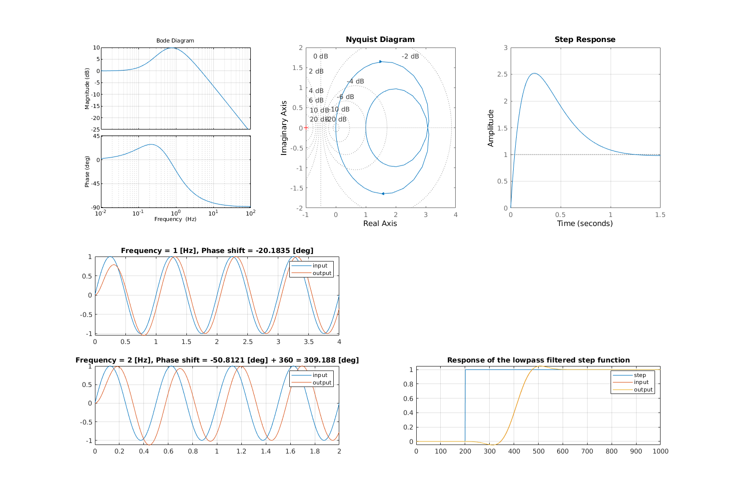
Minium phase system with large overshoot

Example 1. [smaller order]

Minimum phase system, which has a very high overshoot. If we remove the high frequency components from the step function, we obtain a beautiful transient.

syms s

b = [1 3 2];
a = poly([ -3 -4 -5 ]);

H = tf(b,a);
DC_gain = dcgain(H);

H = H / DC_gain;
H_sym = poly2sym(b,s)/poly2sym(a,s) / DC_gain;
H_fh = matlabFunction(H_sym);

if exist('fig2','var')
    delete(fig2)
end

fig2 = figure(2);
set(fig2, 'Position', [ 383 2 1461 1000 ], 'Color', [1 1 1])

subplot(231),
bopts = bodeoptions;
bopts.FreqUnits = 'Hz';
bodeplot(H,bopts), grid on

subplot(232), nyquist(H), grid on

subplot(233), step(H), grid on

subplot(425);

f = 1;
w = 2*pi*f;
t = linspace(0,4/f,500);
u = sin(w*t);

absHw = abs(H_fh(1i*w));
argHw = angle(H_fh(1i*w)) / pi * 180;

y = lsim(H,u,t) / absHw;

plot(t,u), hold on
plot(t,y), grid on
title(sprintf('Frequency = %g [Hz], Phase shift = %g [deg]', f, argHw))
legend input output

subplot(427);

f = 2;
w = 2*pi*f;
t = linspace(0,4/f,500);
u = sin(w*t);

absHw = abs(H_fh(1i*w));
argHw = angle(H_fh(1i*w)) / pi * 180;

y = lsim(H,u,t) / absHw;

plot(t,u), hold on
plot(t,y), grid on
title(sprintf('Frequency = %g [Hz], Phase shift = %g [deg] + 360 = %g [deg]', f, argHw, argHw + 360))
legend input output


% Lowpass filter design
% openExample('dsp/LowpassFilterDesignExample')
N   = 420;
Fs  = 1;
Fp  = 2e-3;
Ap  = 0.1;
Ast = 80;

Rp  = (10^(Ap/20) - 1)/(10^(Ap/20) + 1);
Rst = 10^(-Ast/20);

window = firceqrip(N,Fp/(Fs/2),[Rp Rst],'passedge');
% fvtool(window,'Fs',Fs);

subplot(428);

T = 1000;
Ts = 1/Fs;
t = 0:Ts:T;
u_step = double( t > T/5 );
u = filter(window,1,u_step);
y = lsim(H,u,t);

plot(t,u_step), hold on
plot(t,u), hold on
plot(t,y), grid on
title('Response of the lowpass filtered step function')
legend step input output

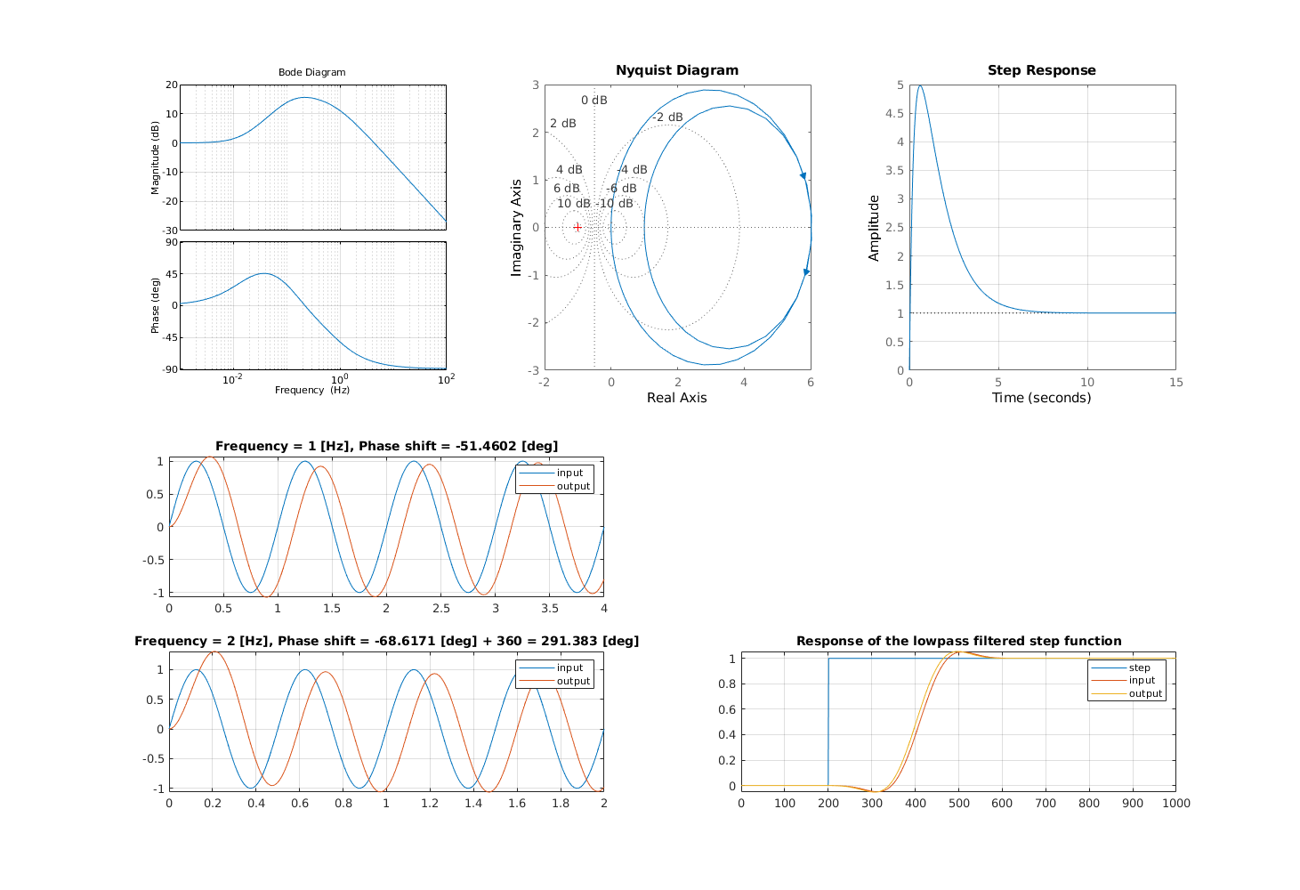
Example 2. [higher order]

syms s

b = poly([-0.1 -2 -3.1 -4.2 -2]);
a = poly([-1.1 -2.2 -1 -3 -4 -5 ]);

H = tf(b,a);
DC_gain = dcgain(H);

H = H / DC_gain;
H_sym = poly2sym(b,s)/poly2sym(a,s) / DC_gain;
H_fh = matlabFunction(H_sym);

if exist('fig2','var')
    delete(fig2)
end

fig2 = figure(2);
set(fig2, 'Position', [ 383 2 1461 1000 ], 'Color', [1 1 1])

subplot(231),
bopts = bodeoptions;
bopts.FreqUnits = 'Hz';
bodeplot(H,bopts), grid on

subplot(232), nyquist(H), grid on

subplot(233), step(H), grid on

subplot(425);

f = 1;
w = 2*pi*f;
t = linspace(0,4/f,500);
u = sin(w*t);

absHw = abs(H_fh(1i*w));
argHw = angle(H_fh(1i*w)) / pi * 180;

y = lsim(H,u,t) / absHw;

plot(t,u), hold on
plot(t,y), grid on
title(sprintf('Frequency = %g [Hz], Phase shift = %g [deg]', f, argHw))
legend input output

subplot(427);

f = 2;
w = 2*pi*f;
t = linspace(0,4/f,500);
u = sin(w*t);

absHw = abs(H_fh(1i*w));
argHw = angle(H_fh(1i*w)) / pi * 180;

y = lsim(H,u,t) / absHw;

plot(t,u), hold on
plot(t,y), grid on
title(sprintf('Frequency = %g [Hz], Phase shift = %g [deg] + 360 = %g [deg]', f, argHw, argHw + 360))
legend input output


% Lowpass filter design
% openExample('dsp/LowpassFilterDesignExample')
N   = 420;
Fs  = 1;
Fp  = 2e-3;
Ap  = 0.1;
Ast = 80;

Rp  = (10^(Ap/20) - 1)/(10^(Ap/20) + 1);
Rst = 10^(-Ast/20);

window = firceqrip(N,Fp/(Fs/2),[Rp Rst],'passedge');
% fvtool(window,'Fs',Fs);

subplot(428);

T = 1000;
Ts = 1/Fs;
t = 0:Ts:T;
u_step = double( t > T/5 );
u = filter(window,1,u_step);
y = lsim(H,u,t);

plot(t,u_step), hold on
plot(t,u), hold on
plot(t,y), grid on
title('Response of the lowpass filtered step function')
legend step input output

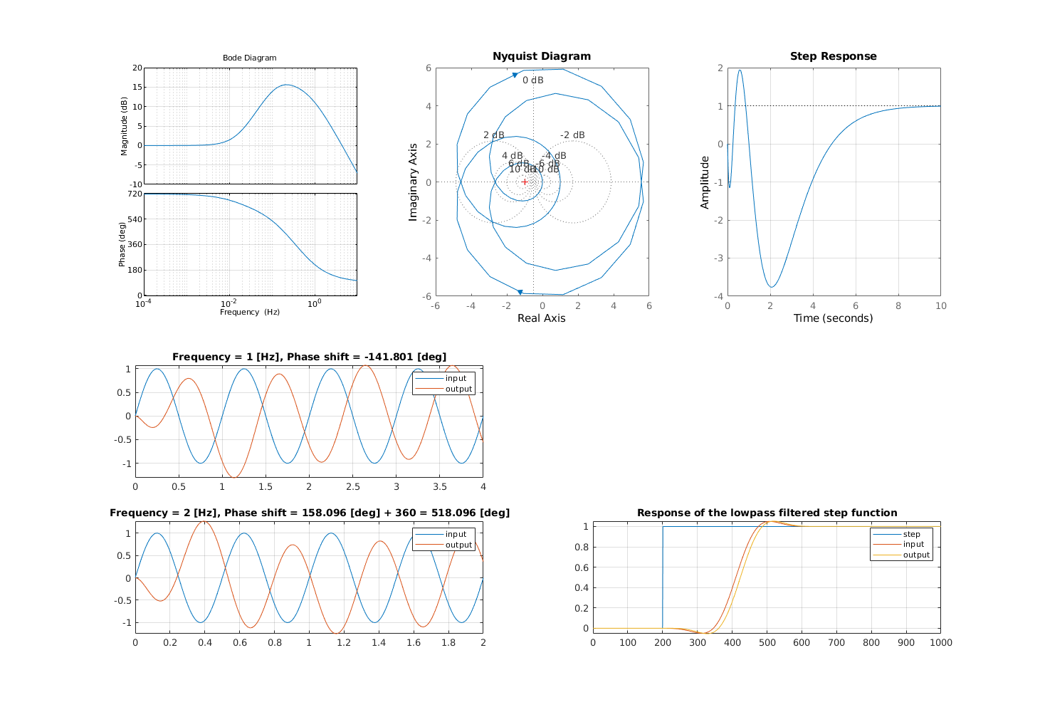
Non-minimum phase system

Example 1

syms s

b = poly([0.1 -2 -3.1 -4.2 -2]);
a = poly([-1.1 -2.2 -1 -3 -4 -5 ]);

H = tf(b,a);
DC_gain = dcgain(H);

H = H / DC_gain;
H_sym = poly2sym(b,s)/poly2sym(a,s) / DC_gain;
H_fh = matlabFunction(H_sym);

if exist('fig2','var')
    delete(fig2)
end

fig2 = figure(2);
set(fig2, 'Position', [ 383 2 1461 1000 ], 'Color', [1 1 1])

subplot(231),
bopts = bodeoptions;
bopts.FreqUnits = 'Hz';
bodeplot(H,bopts), grid on

subplot(232), nyquist(H), grid on

subplot(233), step(H), grid on

subplot(425);

f = 1;
w = 2*pi*f;
t = linspace(0,4/f,500);
u = sin(w*t);

absHw = abs(H_fh(1i*w));
argHw = angle(H_fh(1i*w)) / pi * 180;

y = lsim(H,u,t) / absHw;

plot(t,u), hold on
plot(t,y), grid on
title(sprintf('Frequency = %g [Hz], Phase shift = %g [deg]', f, argHw))
legend input output

subplot(427);

f = 2;
w = 2*pi*f;
t = linspace(0,4/f,500);
u = sin(w*t);

absHw = abs(H_fh(1i*w));
argHw = angle(H_fh(1i*w)) / pi * 180;

y = lsim(H,u,t) / absHw;

plot(t,u), hold on
plot(t,y), grid on
title(sprintf('Frequency = %g [Hz], Phase shift = %g [deg] + 360 = %g [deg]', f, argHw, argHw + 360))
legend input output


% Lowpass filter design
% openExample('dsp/LowpassFilterDesignExample')
N   = 420;
Fs  = 1;
Fp  = 2e-3;
Ap  = 0.1;
Ast = 80;

Rp  = (10^(Ap/20) - 1)/(10^(Ap/20) + 1);
Rst = 10^(-Ast/20);

window = firceqrip(N,Fp/(Fs/2),[Rp Rst],'passedge');
% fvtool(window,'Fs',Fs);

subplot(428);

T = 1000;
Ts = 1/Fs;
t = 0:Ts:T;
u_step = double( t > T/5 );
u = filter(window,1,u_step);
y = lsim(H,u,t);

plot(t,u_step), hold on
plot(t,u), hold on
plot(t,y), grid on
title('Response of the lowpass filtered step function')
legend step input output

Example 2

syms s

b = poly([0.1 2 3.1 -4.2 -2]);
a = poly([-1.1 -2.2 -1 -3 -4 -5 ]);

H = tf(b,a);
DC_gain = dcgain(H);

H = H / DC_gain;
H_sym = poly2sym(b,s)/poly2sym(a,s) / DC_gain;
H_fh = matlabFunction(H_sym);

if exist('fig2','var')
    delete(fig2)
end

fig2 = figure(2);
set(fig2, 'Position', [ 383 2 1461 1000 ], 'Color', [1 1 1])

subplot(231),
bopts = bodeoptions;
bopts.FreqUnits = 'Hz';
bodeplot(H,bopts), grid on

subplot(232), nyquist(H), grid on

subplot(233), step(H), grid on

subplot(425);

f = 1;
w = 2*pi*f;
t = linspace(0,4/f,500);
u = sin(w*t);

absHw = abs(H_fh(1i*w));
argHw = angle(H_fh(1i*w)) / pi * 180;

y = lsim(H,u,t) / absHw;

plot(t,u), hold on
plot(t,y), grid on
title(sprintf('Frequency = %g [Hz], Phase shift = %g [deg]', f, argHw))
legend input output

subplot(427);

f = 2;
w = 2*pi*f;
t = linspace(0,4/f,500);
u = sin(w*t);

absHw = abs(H_fh(1i*w));
argHw = angle(H_fh(1i*w)) / pi * 180;

y = lsim(H,u,t) / absHw;

plot(t,u), hold on
plot(t,y), grid on
title(sprintf('Frequency = %g [Hz], Phase shift = %g [deg] + 360 = %g [deg]', f, argHw, argHw + 360))
legend input output


% Lowpass filter design
% openExample('dsp/LowpassFilterDesignExample')
N   = 420;
Fs  = 1;
Fp  = 2e-3;
Ap  = 0.1;
Ast = 80;

Rp  = (10^(Ap/20) - 1)/(10^(Ap/20) + 1);
Rst = 10^(-Ast/20);

window = firceqrip(N,Fp/(Fs/2),[Rp Rst],'passedge');
% fvtool(window,'Fs',Fs);

subplot(428);

T = 1000;
Ts = 1/Fs;
t = 0:Ts:T;
u_step = double( t > T/5 );
u = filter(window,1,u_step);
y = lsim(H,u,t);

plot(t,u_step), hold on
plot(t,u), hold on
plot(t,y), grid on
title('Response of the lowpass filtered step function')
legend step input output

Output:

└ 10.3037 [sec]

Published with MATLAB® R2018a, and sanitarized by BeautifulSoup (Python script using BSoup is written by Polcz).