Polcz Péter honlapja

Ezt a példát a MathWorks oldaláról töltöttem le és írtam át demonstráció végett.

This example shows how to solve a nonlinear elliptic problem numerically, using the pdenonlin function in Partial Differential Equation Toolbox™. In many problems, the coefficients not only depend on spatial coordinates, but also on the solution itself. In toolbox wording, this kind of problem is called nonlinear. An example of this is the minimal surface equation.

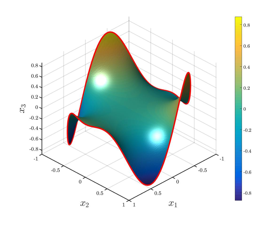
We envision to minimize the surface of a two-variable function $u:S \to \mathbf{R}$, namely $$ I(u) = \iint_S ~~ \underbrace{ \sqrt{1 + (u'_x)^2 + (u'_y)^2} }_{F(\not x, \not u, u'_x, u'_y)} ~~ \mathrm{d}(x,y) \to \mathrm{min} $$ The Euler-Lagrange equation will look like: $$ \frac{\partial}{\partial x} \left( \frac{\partial F}{\partial u'_x} \right) + \frac{\partial}{\partial y} \left( \frac{\partial F}{\partial u'_y} \right) = \frac{\partial}{\partial x} \left( \frac{u'_x}{\sqrt{1 + (u'_x)^2 + (u'_y)^2}} \right) + \frac{\partial}{\partial y} \left( \frac{u'_y}{\sqrt{1 + (u'_x)^2 + (u'_y)^2}} \right) = 0 $$ We can reformulate the equation as follows: $$-\nabla \cdot \left( \frac{1}{\sqrt{1 + \left|\nabla u\right|^2}} \nabla u \right) = 0$$ We solve this equation on the unit disk, with $u(x,y) = \sin(3x)\cos(3y)$ for all $(x,y) \in \partial S$ boundary condition. The PDE coefficient c is the multiplier of $\nabla u$, namely $$\frac{1}{\sqrt{1 + \left|\nabla u\right|^2}}$$ c is a function of the solution $u$, so the problem is nonlinear.

Problem Definition
Geommetry
Boundary Conditions
Generate Mesh
Solve PDE
Plot Solution

Problem Definition

The following variables define the problem:

information, see the documentation page for circleg and pdegeom. * c, a, f: The coefficients of the PDE. Note that c is a character array. For more information on passing coefficients into pdenonlin, see the documentation page for assempde. * rtol: Tolerance for nonlinear solver.

c = '1./sqrt(1+ux.^2+uy.^2)';
a = 0;
f = 0;
rtol = 1e-3;

Geommetry

% Create a PDE Model with a single dependent variable
numberOfPDE = 1;
pdem = createpde(numberOfPDE);

% Create a geometry entity and append to the pde model
pdeGeom = @circleg;
geometryFromEdges(pdem,pdeGeom);

% Plot the geometry and display the edge labels for use in the boundary condition definition.
figure;
pdegplot(pdem, 'edgeLabels', 'on');
axis equal
title 'Geometry With Edge Labels Displayed';

Boundary Conditions

bc_fh = @(x,y) sin(3*x).*cos(3*y);
bcFunc = @(thePde, loc, state) bc_fh(loc.x,loc.y);
applyBoundaryCondition(pdem,'Edge',(1:4), 'u', bcFunc);

Generate Mesh

msh = generateMesh(pdem,'Hmax',0.02);
figure;
pdemesh(pdem);
axis equal

Solve PDE

Because the problem is nonlinear, we solve it using the pdenonlin function.

u = pdenonlin(pdem,c,a,f,'tol',rtol, 'Jacobian', 'full', 'Report', 'on');

Iteration     Residual     Step size  Jacobian: full
   0          3.6280e-02
   1          3.0928e-03   1.0000000
   2          3.3439e-04   1.0000000

Plot Solution

% Ennek segitsegevel lehet visszakerni a celtartomany hatarainak koordinatait
figure,
h = pdegplot(pdeGeom);
x1 = h.XData;
x2 = h.YData;
delete(h), close;

% Koordinata rendszer kialakitasa, stb...
fig = figure('InvertHardcopy','off','Color',[1 1 1], ...
    'Units', 'normalized', 'Position', [0 0 0.6 1]);
ax = axes('Parent',fig,'LineWidth',2,'FontSize',16,...
    'FontName','TeX Gyre Schola Math',...
    'DataAspectRatio',[1 1 1]);
hold(ax, 'on');
axis(ax, 'tight');
colorbar,
light('Parent', ax)
view(ax,[135,32]);
grid(ax,'on');
xlabel('$x_1$','FontSize',30,'Interpreter','latex');
ylabel('$x_2$','FontSize',30,'Interpreter','latex');
zlabel('$x_3$','FontSize',30,'Interpreter','latex');

% Felulet kirajzolasa
trisurf(msh.Elements', msh.Nodes(1,:)', msh.Nodes(2,:)', u, 'facealpha', 1);
shading interp

% Drotkeret kirajzolasa
plot3(x1,x2,bc_fh(x1,x2), 'r', 'LineWidth', 4)

Tartalomjegyzék