Tartalomjegyzék

Meaning of involutive distribution

Teljes Matlab script kiegészítő függvényekkel.

File: involutive.m
Directory: 4_gyujtemegy/11_CCS/_2_nonlin-pannon/2018
Author: Peter Polcz (ppolcz@gmail.com)

Created on 2018. July 27.

Inherited from

file:   nonlin_distributions_coordinate_systems.m
author: Peter Polcz <ppolcz@gmail.com>

Created on 2017.06.04. Sunday, 14:57:05

Requires

vekanal_subsmesh.m

Canonic basis vectors in polar coordinates

syms x y theta r real
assumeAlso(in(r,'positive'))

r = [x;y];
r_prime = [r;theta];

R = [sqrt(x^2 + y^2) ; atan(y/x) ];
J = jacobian(R, r);

Rp = [r*cos(theta) ; r*sin(theta)];
Jp = jacobian(Rp, r_prime);

% simplify(subs(simplify(subs(Jp * J, Zi, Rp)), sign(r), 1))
% simplify(subs(simplify(subs(Jp * J, Zip, R)), sign(r), 1))

f_sym = [
    -y
    x
    ];

g_sym = [
    x
    y
    ] / sqrt(x^2 + y^2);

br_fg = simplify(jacobian(g_sym,r)*f_sym - jacobian(f_sym,r)*g_sym)

f_fh = matlabFunction(f_sym,'vars',{'t' r});
g_fh = matlabFunction(g_sym,'vars',{'t' r});

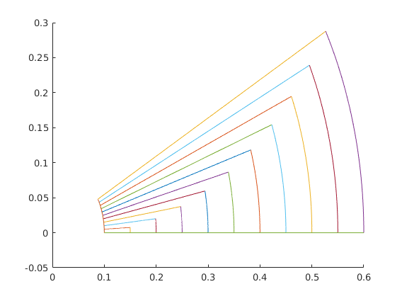
figure, hold on
for h = linspace(0.05,0.5,10)
    x0 = [0.1,0];
    N = 1000;
    [~,p1] = ode45(f_fh, linspace(0,h,N), x0);
    [~,p2] = ode45(g_fh, linspace(0,h,N), p1(end,:)');
    [~,p3] = ode45(@(t,x) -f_fh(-t,x), linspace(0,h,N), p2(end,:)');
    [~,p4] = ode45(@(t,x) -g_fh(-t,x), linspace(0,h,N), p3(end,:)');

    plot(p1(:,1),p1(:,2)),
    plot(p2(:,1),p2(:,2)),
    plot(p3(:,1),p3(:,2)),
    plot(p4(:,1),p4(:,2)),
end

Output:

br_fg =
 0
 0

vekanal_quiver_sym(f_sym, r, {0,1,20}, {0,1,20})
vekanal_quiver_sym(g_sym, r, {0,1,20}, {0,1,20})

Output:

ans = 
  Quiver with properties:

        Color: [0.3010 0.7450 0.9330]
    LineStyle: '-'
    LineWidth: 0.5000
        XData: [20×20 double]
        YData: [20×20 double]
        ZData: []
        UData: [20×20 double]
        VData: [20×20 double]
        WData: []

  Use GET to show all properties
ans = 
  Quiver with properties:

        Color: [0.6350 0.0780 0.1840]
    LineStyle: '-'
    LineWidth: 0.5000
        XData: [20×20 double]
        YData: [20×20 double]
        ZData: []
        UData: [20×20 double]
        VData: [20×20 double]
        WData: []

  Use GET to show all properties

Cycloid coordinate system

syms x y t r real
assume(in(r,'real') | in(r,'positive'))

Z = [x;y];
Zp = [r;t];

R = [
    r*(t-sin(t))
    r*(1-cos(t))
    ];

J = jacobian(R,Zp)

Output:

J =
[ t - sin(t), -r*(cos(t) - 1)]
[ 1 - cos(t),        r*sin(t)]

syms x1 x2 x3 real
x = [x1;x2;x3];

tau1 = [
    cos(x3)
    sin(x3)
    0
    ];
tau2 = [
    0
    0
    1
    ];

jacobian(tau2,x)*tau1 - jacobian(tau1,x)*tau2


f_sym = @(t,x) [
    sin(x(1))
    cos(x(2))
    ];
g_sym = @(t,x) [
    -cos(x(1))
    sin(x(2))
    ];

figure, hold on
for h = linspace(0.05,0.5,10)
    x0 = [1,1];
    N = 1000;
    [~,p1] = ode45(f_sym, linspace(0,h,N), x0);
    [~,p2] = ode45(g_sym, linspace(0,h,N), p1(end,:)');
    [~,p3] = ode45(@(t,x) -f_sym(-t,x), linspace(0,h,N), p2(end,:)');
    [~,p4] = ode45(@(t,x) -g_sym(-t,x), linspace(0,h,N), p3(end,:)');

    plot(p1(:,1),p1(:,2)),
    plot(p2(:,1),p2(:,2)),
    plot(p3(:,1),p3(:,2)),
    plot(p4(:,1),p4(:,2)),
end

Output:

ans =
  sin(x3)
 -cos(x3)
        0

Published with MATLAB® R2017a, and sanitarized by BeautifulSoup (Python script using BSoup is written by Polcz).