Tartalomjegyzék
\[ \newenvironment{dcases}{\left\{\begin{array}{ll}}{\end{array}\right.} \]Script integral_curves_of_electric_field
TELJES MATLAB SCRIPT KIEGÉSZÍTŐ FÜGGVÉNYEKKEL
file:   integral_curves_of_electric_field.m
author: Peter Polcz <ppolcz@gmail.com>
Created on 2017.07.02. Sunday, 03:39:45
Output:
┌integral_curves_of_electric_field
│   - Persistence for `integral_curves_of_electric_field` reused (inherited) [run ID: 7354, 2017.08.27. Sunday, 04:03:07]
│   - Script `integral_curves_of_electric_field` backuped
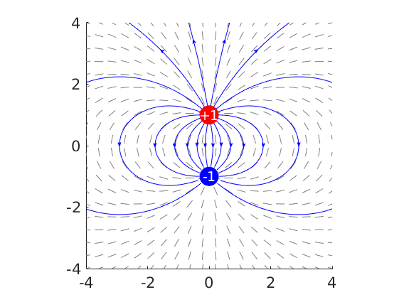
Integral slopes and curves of the electric dipole
Q1 = 1;
r1 = [0;1];

Q2 = -1;
r2 = [0;-1];

F = @(t,r) Q1*(r-r1) / norm(r-r1)^3 + Q2*(r-r2) / norm(r-r2)^3;
Fn = @(t,r) F(t,r) / norm(F(t,r));

g = 4;
figure, hold on

[x,y] = meshgrid(linspace(-g,g,20));
dx = 0*x;
dy = 0*y;
for i = 1:numel(x);
    Fi = F(0,[x(i);y(i)]);
    dx(i) = Fi(1);
    dy(i) = Fi(2);
end
pcz_integral_slopes(x,y,dx,dy,'Color',0.5*[1 1 1])

R = 0.3;
t = linspace(0,pi,10);
t = [t -t];
X = R*cos(t) + r1(1);
Y = R*sin(t) + r1(2);

for i = 1:numel(X)
    ri = [X(i);Y(i)];

    tt = 0;
    xx = ri';
    for k = 1:10000
        [t_ode,x_ode] = ode45(Fn,[0,0.1],ri);
        tt = [tt ; t_ode(2:end,:)];
        xx = [xx ; x_ode(2:end,:)];

        last = find(sum((x_ode - repmat(r2',[size(x_ode,1),1])).^2,2) < R^2,1);
        if ~isempty(last)
            break;
        end

        if norm(x_ode(end,:)) > g*sqrt(2), break; end

        ri = x_ode(end,:)';
    end

    % Canonic parametrization of the curve
    s = [ 0 ; cumsum(sum(diff(xx,1).^2,2).^0.5) ];
    p = interp1(s,xx,s(end)/2);
    q = interp1(s,xx,s(end)/2+0.01);
    pcz_arrow(p(1),p(2),q(1),q(2),'Color','blue','HeadLength',4,'HeadWidth',4);
    % quiver(p(1),p(2),q(1)-p(1),q(2)-p(2),'Color','blue')

    xx = interp1(s,xx,0:0.1:s(end));
    plot(xx(:,1),xx(:,2),'b')

    drawnow
end

s = {'' '' '+'};

% plot(r1(1),r1(2),'r.','MarkerSize',60);
% plot(r2(1),r2(2),'b.','MarkerSize',60);

rectangle('Position',[r1(1)-R,r1(2)-R,2*R,2*R],'Curvature',[1,1],...
    'FaceColor','red','EdgeColor','red');
rectangle('Position',[r2(1)-R,r2(2)-R,2*R,2*R],'Curvature',[1,1],...
    'FaceColor','blue','EdgeColor','blue');

text(r1(1),r1(2),[s{sign(Q1)+2} num2str(Q1)],'HorizontalAlignment','center','Color','white','FontSize',14)
text(r2(1),r2(2),[s{sign(Q2)+2} num2str(Q2)],'HorizontalAlignment','center','Color','white','FontSize',14)

axis equal
axis([-g g -g g])

set(gca,'fontsize',16)
pcz_print dipole.png -r100
Output:
│   - File saved to:
dipole.png
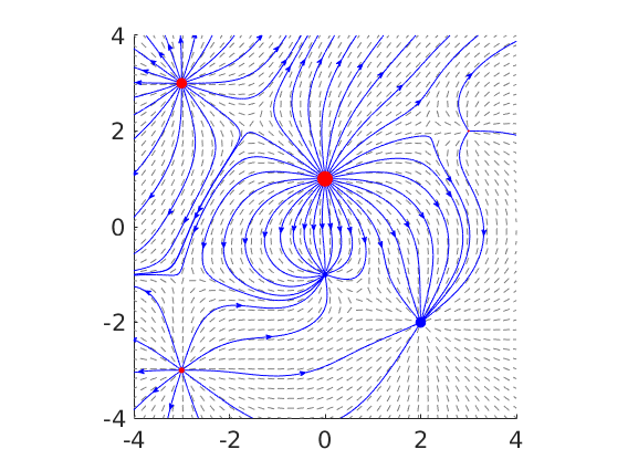
Integral slopes and curves of the electric multipole
Qp = [ 3 2 1 0.3];
rp = [
    0 -3 -3 3
    1  3 -3 2
    ];

Qn = [ -1 -2 ];
rn = [
     0  2
    -1 -2
    ];

Qs = [Qp Qn];
rs = [rp rn];

n = numel(Qs);

sqrtdist = @(r) sum((r(:,ones(1,n))-rs).^2,1);
F = @(t,r) sum(Qs([1,1],:).*(r(:,ones(1,n))-rs) ./ repmat(sqrtdist(r).^(3/2),[2 1]),2);
Fn = @(t,r) F(t,r) / norm(F(t,r));

g = 4;
fig = figure; hold on

[x,y] = meshgrid(linspace(-g,g,40));
dx = 0*x;
dy = 0*y;
for i = 1:numel(x);
    Fi = F(0,[x(i);y(i)]);
    dx(i) = Fi(1);
    dy(i) = Fi(2);
end
pcz_integral_slopes(x,y,dx,dy,'Color',0.5*[1 1 1])

R_divider = 20;
X = [];
Y = [];
for i = 1:numel(Qp)
    R = abs(Qp(i))/R_divider;
    t = linspace(0,2*pi,round(Qp(i)*10)+1);
    X = [ X R*cos(t(2:end)) + rp(1,i) ];
    Y = [ Y R*sin(t(2:end)) + rp(2,i) ];
end

for i = 1:numel(X)
    ri = [X(i);Y(i)];

    tt = 0;
    xx = ri';
    for k = 1:1000
        [t_ode,x_ode] = ode45(@(t,x) Fn(t,x),[0,0.1],ri);
        tt = [tt ; t_ode(2:end,:)];
        xx = [xx ; x_ode(2:end,:)];

        found = 0;
        for j = 1:numel(Qn)
            last = find(sum((x_ode - repmat(rn(:,j)',[size(x_ode,1),1])).^2,2) < 0.01,1);
            if ~isempty(last)
                found = 1;
                break;
            end
        end
        if found, break; end

        % norm(x_ode(end,:))
        if norm(x_ode(end,:)) > g*sqrt(2), break; end

        ri = x_ode(end,:)';
    end

    % Canonic parametrization of the curve
    s = [ 0 ; cumsum(sum(diff(xx,1).^2,2).^0.5) ];
    p = interp1(s,xx,s(end)/2,'spline');
    q = interp1(s,xx,s(end)/2+0.01,'spline');
    pcz_arrow(p(1),p(2),q(1),q(2),'Color','blue','HeadLength',4,'HeadWidth',4);

    plot(xx(:,1),xx(:,2),'b')

    drawnow
end

% s = {'' '' '+'};
% for i = 1:n
%     if Qs(i) > 0
%         color = 'r.';
%     else
%         color = 'b.';
%     end
%     plot(rs(1,i),rs(2,i),color,'MarkerSize',60);
%     text(rs(1,i),rs(2,i),[s{sign(Qs(i))+2} num2str(Qs(i))],...
%         'HorizontalAlignment','center','Color','white','FontSize',8)
% end

s = {'' '' '+'};
for i = 1:n
    if Qs(i) > 0
        color = 'r';
    else
        color = 'b';
    end
    R = abs(Qs(i))/R_divider;
    rectangle('Position',[rs(1,i)-R,rs(2,i)-R,2*R,2*R],'Curvature',[1,1],...
        'FaceColor',color,'EdgeColor',color);
end

axis equal
axis([-g g -g g])

set(gca,'fontsize',16)
pcz_print multipole.png -r200
Output:
│   - File saved to:
multipole.png
Demonstrációs céllal
headWidth = 8;
headLength = 8;
LineLength = 0.08;

%some data
[x,y] = meshgrid(0:0.2:2,0:0.2:2);
u = cos(x).*y;
v = sin(x).*y;

%quiver plots
figure('Position',[10 10 1000 600],'Color','w');
hax_1 = subplot(1,2,1);
hq = quiver(x,y,u,v);           %get the handle of quiver
title('Regular Quiver plot','FontSize',16);

%get the data from regular quiver
U = hq.UData;
V = hq.VData;
X = hq.XData;
Y = hq.YData;

%right version (with annotation)
hax_2 = subplot(1,2,2);
%hold on;
for ii = 1:length(X)
    for ij = 1:length(X)

        headWidth = 5;
        ah = annotation('arrow',...
            'headStyle','cback1','HeadLength',headLength,'HeadWidth',headWidth);
        set(ah,'parent',gca);
        set(ah,'position',[X(ii,ij) Y(ii,ij) LineLength*U(ii,ij) LineLength*V(ii,ij)]);

    end
end
%axis off;
title('Quiver - annotations ','FontSize',16);

linkaxes([hax_1 hax_2],'xy');

End of the script.
Output:
└ 34.077 [sec]