Tartalomjegyzék

CCS 2017b Gyak 3. Frekvenciatartomány

Teljes Matlab script (és live script) kiegészítő függvényekkel.
Tekintsd meg LiveEditor nézetben is!

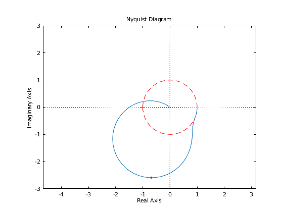
Egy egyszeru pelda arra, amikor a fazistartalek negativ

s = tf('s');
H = (0.5*s + 1) / (8*s^3 + 4*s^2 + 3*s + 1)
[Gm,Pm,Wgm,Wpm] = margin(H)
figure, hold on
fplot(@(t) sqrt(1 - t.^2),[-1 1], 'r--')
fplot(@(t) -sqrt(1 - t.^2),[-1 1], 'r--')
Ny_opts = nyquistoptions;
Ny_opts.ShowFullContour = 'off';
Ny_opts.Grid = 'off';
Ny_opts.MagUnits = 'abs';
nyquistplot(H, Ny_opts), axis equal
figure, hold on
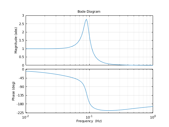
Bd_opts = bodeoptions;
Bd_opts.FreqUnits = 'Hz';
Bd_opts.FreqScale = 'log';
Bd_opts.MagUnits = 'abs';
bodeplot(H,Bd_opts), grid on
xlim([0.01,1])

Output:

H =
 
         0.5 s + 1
  -----------------------
  8 s^3 + 4 s^2 + 3 s + 1
 
Continuous-time transfer function.

Gm =
    0.6667
Pm =
  -12.5307
Wgm =
    0.6455
Wpm =
    0.6895

Visszacsatolt zárt hurok

H_cls = feedback(H,1);
[Poles, Zeros] = pzmap(H_cls)
figure('Position', [ 211 81 583 437 ], 'Color', [1 1 1])
bodeplot(H_cls, Bd_opts)
xlim([0.01,1])

Output:

Poles =
   0.0213 + 0.6784i
   0.0213 - 0.6784i
  -0.5427 + 0.0000i
Zeros =
    -2

hann

Published with MATLAB® R2017b, and sanitarized by BeautifulSoup (Python script using BSoup is written by Polcz).