Tartalomjegyzék
\[ \newenvironment{dcases}{\left\{\begin{array}{ll}}{\end{array}\right.} \]Feedback linearization
Teljes Matlab script kiegészítő függvényekkel.
File: Isidori_reldegree_coord_trafo.m
Directory: 4_gyujtemegy/11_CCS/_2_nonlin-pannon/2018
Author: Peter Polcz (ppolcz@gmail.com)
Created on 2018. July 29.
Isidori I., Example 4.1.4
Feedback linearization
syms t u v real
syms x1 x2 x3 real
syms z1 z2 z3 real

x = [x1 ; x2 ; x3];
z = [z1 ; z2 ; z3];

d = @(g) jacobian(g,x);
Lie = @(f,g) d(g)*f;
br = @(f,g) d(g)*f - d(f)*g;

f = [ -x1 ; x1*x2 ; x2 ];
g = [ exp(x2) ; 1 ; 0 ];
h = x3;

phi3 = 1 + x1 - exp(x2);

Phi = [
    h
    Lie(f,h)
    phi3
    ];

% Quick check: should be zero
% Lie(g,phi3)
Quick check
\begin{align}L_g \phi_3(x) = 0\end{align}$\phi_3(x)$-et Isidori hasraütés szerűen adta meg, de jól látható, hogy az tényleg jó megoldás és a Mathematica-val is ki lehet számolni.
Phi_inv = struct2cell(solve(z-Phi, x1, x2, x3));
Phi_inv = [ Phi_inv{:} ]';
Coordinate transformation
b = Lie(f, Lie(f,h));
a = Lie(g, Lie(f,h));
q3 = Lie(f, Phi(3));
b = subs(b, x, Phi_inv);
a = subs(a, x, Phi_inv);
q3 = subs(q3, x, Phi_inv);
dz = simplify([ z2 ; collect(b+a*u,u) ; q3 ]);
System dynamics in the new coordinates
\begin{align}\dot z = \left(\begin{array}{c} z_{2}\\ u+z_{2}\,\left(z_{3}+{\mathrm{e}}^{z_{2}}-1\right)\\ -\left(z_{2}\,{\mathrm{e}}^{z_{2}}+1\right)\,\left(z_{3}+{\mathrm{e}}^{z_{2}}-1\right) \end{array}\right)\end{align}Linearizing feedback design
u_fdb = a \ (-b + v);
Closed loop
dz_fdb = simplify(subs(dz, u, u_fdb));
Zero dynamics
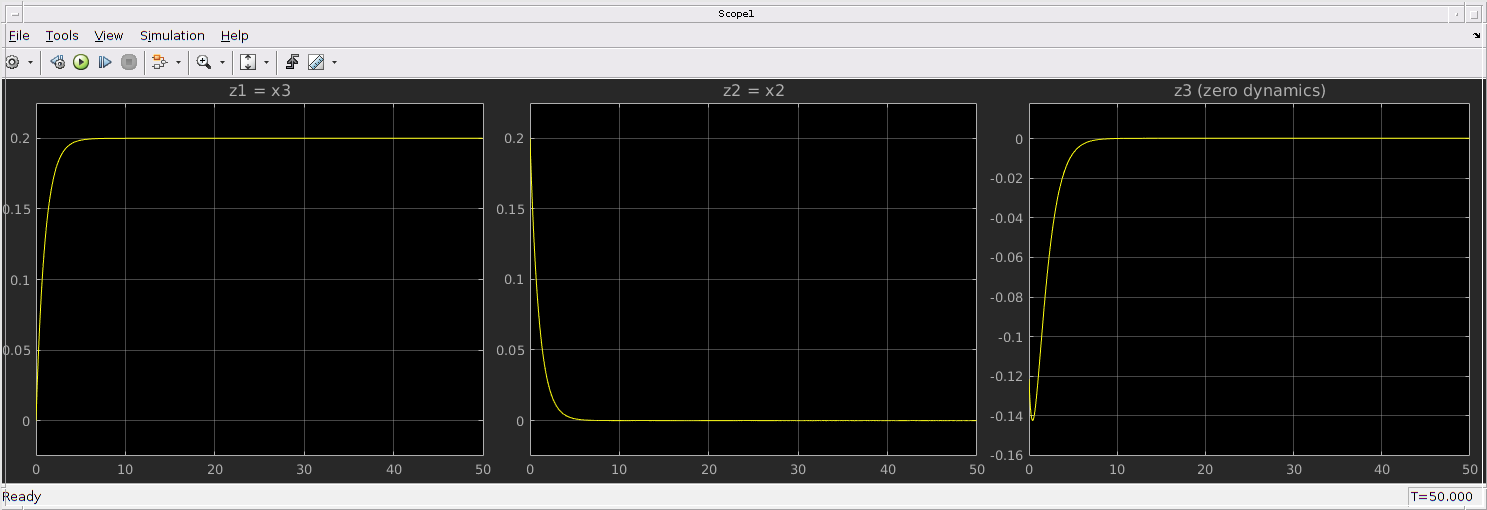
Zero_dynamics = simplify(subs(dz_fdb, [z1 z2 v], [0 0 0]));
The zero dynamics is stable in the origin.
\begin{align}\dot z_3 = -z_{3}\end{align}Linearized dynamics
Overall dynamics without the zero dynamics.
A = [
    0 1
    0 0
    ];

B = [
    0
    1
    ];

C = [ 1 0 ];

sys = ss(A,B,C,0);

s = tf('s');

H = tf(sys)

eps1 = 0.01;
eps2 = 0.01;

H_control = s^2/(eps1*s^2 + eps2*s + 1);

He = minreal(feedback(H*H_control,1))

[POLES, ZEROS] = pzmap(He)
Output:
H =

   1
  ---
  s^2

Continuous-time transfer function.


He =

       100
  -------------
  s^2 + s + 200

Continuous-time transfer function.

POLES =
  -0.5000 +14.1333i
  -0.5000 -14.1333i
ZEROS =
  0×1 empty double column vector
PID controller for the linearized dynamics
Download model here: Isidori_Example414_PID.slx
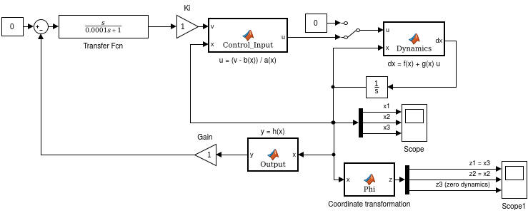
open_system Isidori_Example414_PID.slx
print -dpng fig/Isidori_Example414_PID.png -sIsidori_Example414_PID

sim Isidori_Example414_PID

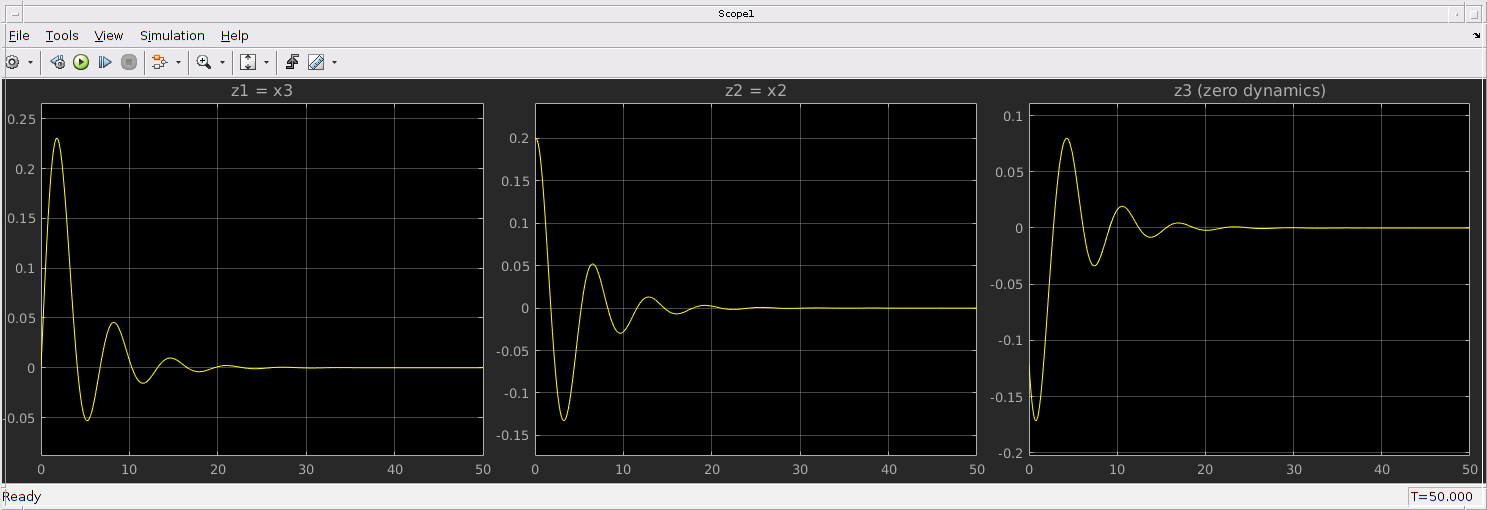
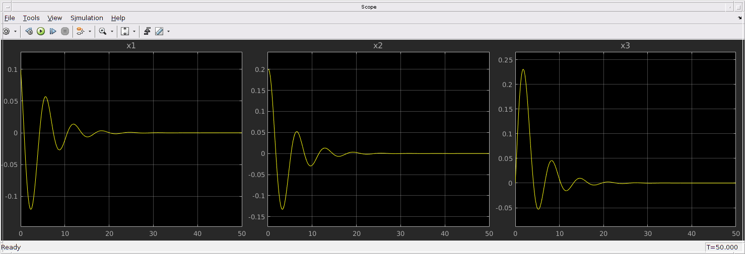
Observer + State feedback
Download model here: Isidori_Example414_obs_state_feedback.slx

% Observer for integrator chain
L = place(A',C',[-2 -3])';

% State feedback gain for LQR
K = lqr(A,B,0.1*eye(2),1);

open_system Isidori_Example414_obs_state_feedback.slx
print -dpng fig/Isidori_Example414_obs_state_feedback.png -sIsidori_Example414_obs_state_feedback

sim Isidori_Example414_obs_state_feedback
Isidori I., Example 4.1.5
Feedback linearization
% clear all
n = 4;
x0 = zeros(n,1);

syms u v real
eval(pcz_generateSymStateVector(n, 'x'));
eval(pcz_generateSymStateVector(n, 'z'));

d = @(g) jacobian(g,x);
Lie = @(f,g) d(g)*f;
br = @(f,g) d(g)*f - d(f)*g;

f = [ x1*x2-x1^3 ; x1 ; -x3 ; x1^2+x2 ];
g = [ 0 ; 2+2*x3 ; 1 ; 0 ];
h = x4;

A = subs(jacobian(f, x), x, x0);
eig_A = eig(A)'
fx0_Is_an_equilibrium_point = subs(f,x,x0)

h
Lie_gh = Lie(g, h)
Lie_gfh = Lie(g, Lie(f,h))

Phi = [
    h
    Lie(f,h)
    x1
    x3
    ]

dPhi = jacobian(Phi, x);

Phi_inv = struct2cell(solve(z-Phi, x_cell{:}));
Phi_inv = [ Phi_inv{:} ]'

b = subs(  Lie(f, Lie(f,h))  , x, Phi_inv);
a = subs(  Lie(g, Lie(f,h))  , x, Phi_inv);
q3 = subs(  Lie(f, Phi(3)) + Lie(g, Phi(3))*u  , x, Phi_inv);
q4 = subs(  Lie(f, Phi(4)) + Lie(g, Phi(4))*u  , x, Phi_inv);

dz = simplify([ z2 ; b+a*u ; q3 ; q4 ])
y = z1

dz_Ell = simplify([
    z2
    z4 + 2*z4*(z4*(z2 - z4^2)- z4^3) + (2 + 2*z3)*u
    -z3 + u
    z4*(-2*z4^2 + z2)
    ])

% calculate zero dynamics

u_fdb = a \ (-b + v)

dz_fdb = simplify(subs(dz, u, u_fdb))
Zero_dynamics = simplify(subs(dz_fdb, [z1 z2 v], [0 0 0]))
Output:
eig_A =
[ -1, 0, 0, 0]
fx0_Is_an_equilibrium_point =
 0
 0
 0
 0
h =
x4
Lie_gh =
0
Lie_gfh =
2*x3 + 2
Phi =
        x4
 x1^2 + x2
        x1
        x3
Phi_inv =
          z3
 - z3^2 + z2
          z4
          z1
dz =
                                       z2
 - 4*z3^4 + 2*z2*z3^2 + z3 + 2*u + 2*u*z4
                       z3*(- 2*z3^2 + z2)
                                   u - z4
y =
z1
dz_Ell =
                                       z2
 - 4*z4^4 + 2*z2*z4^2 + z4 + 2*u + 2*u*z3
                                   u - z3
                       z4*(- 2*z4^2 + z2)
u_fdb =
(v - z3 + 2*z3*(z3^3 - z3*(- z3^2 + z2)))/(2*z4 + 2)
dz_fdb =
                                                        z2
                                                         v
                                        z3*(- 2*z3^2 + z2)
 (v - z3 + 2*z3*(z3^3 - z3*(- z3^2 + z2)))/(2*z4 + 2) - z4
Zero_dynamics =
                                 0
                                 0
                           -2*z3^3
 - z4 - (- 4*z3^4 + z3)/(2*z4 + 2)