Tartalomjegyzék
\[ \newenvironment{dcases}{\left\{\begin{array}{ll}}{\end{array}\right.} \]Basic linear algebra operations
Teljes Matlab script kiegészítő függvényekkel.
File: ccs_TP_linalg.m
Directory: 4_gyujtemegy/11_CCS/_1_ccs/ccs_2018/TP_2018_09_18
Author: Peter Polcz (ppolcz@gmail.com)
Created on 2018. September 18.
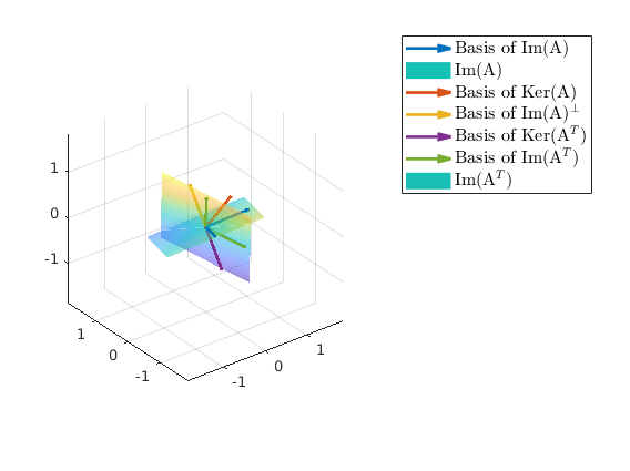
Subspace, image and kernel space
Given an orthonormal basis of the image space of matrix
$$A = \pmqty{ -2 & -1 & 7 \\ -3 & -5 & 14 \\ 1 & 2 & -5 }.$$
A = [
   -2    -1     7
   -3    -5    14
    1     2    -5
    ];

Im = orth(A);

figure;
pcz_plotvec(Im, 'LineWidth', 2, 'DisplayName', 'Basis of Im(A)'), hold on;
pcz_plotplane(Im, 'DisplayName', 'Im(A)', 'FaceAlpha', 0.5)
shading interp
grid on
L = legend;
L.Interpreter = 'latex';
L.FontSize = 12;
Give on orthonormal basis of the kernel (or null) space of matrix $A$.
Ker = null(A);
pcz_plotvec(Ker, 'LineWidth', 2, 'DisplayName', 'Basis of Ker(A)');
Give on orthonormal basis of $\rm{Im}(A)^\perp$, the orthogonal complement of the imaage space of matrix $A$.
ImOrthCo = null(Im');
pcz_plotvec(ImOrthCo, 'LineWidth', 2, 'DisplayName', 'Basis of Im(A)$^\perp$')
Give on orthonormal basis of the kernel space of matrix $A^T$.
KerT = null(A');
pcz_plotvec(KerT, 'LineWidth', 2, 'DisplayName', 'Basis of Ker(A$^T$)');
Given on orthonormal basis of the image space of matrix $A^T$.
ImT = orth(A');
pcz_plotvec(ImT, 'LineWidth', 2, 'DisplayName', 'Basis of Im(A$^T$)');
pcz_plotplane(ImT, 'DisplayName', 'Im(A$^T$)', 'FaceAlpha', 0.5)
shading interp
Compute the sinular value decomposition of matrix $A$.
[U,S,V] = svd(A)
Output:
U =
   -0.4095    0.9030   -0.1302
   -0.8583   -0.3329    0.3906
    0.3093    0.2717    0.9113
S =
   17.6612         0         0
         0    1.4425         0
         0         0    0.0000
V =
    0.2097   -0.3713    0.9045
    0.3012    0.9046    0.3015
   -0.9302    0.2092    0.3015
Compute the rank of diagonal matrix $S$ and matrix $A$.
rank(S), rank(A)
Output:
ans =
     2
ans =
     2
Compute the intersection of $V = \rm{Im}(A)$ and $W = \rm{Im}(A^T)$. Note that $V \cap W = \Big(V^\perp \cup W^\perp\Big)^\perp$
V = orth(A);
W = orth(A');

OrthV = null(V');
OrthW = null(W');

Union_OrthV_OrthW = orth( [ OrthV , OrthW ] );

Intersection_V_W = null(Union_OrthV_OrthW');

figure,
pcz_plotvec(Intersection_V_W, 'LineWidth', 2), hold on;
pcz_plotplane(V, 'FaceAlpha', 0.8);
pcz_plotplane(W, 'FaceAlpha', 0.8);
view([ 160.1 , 29.2 ])
shading interp

Partial fractional decomposition
Using residue.
Example 1.
syms s

b_sym = s;
a_sym = s^2 + 3*s + 2;

H1_sym = b_sym/a_sym;

a = sym2poly(a_sym);
b = sym2poly(b_sym);

[r,p,k] = residue(b,a)

H1_pfrac_sym = sum(r ./ (s - p));
Output:
r =
     2
    -1
p =
    -2
    -1
k =
     []
\begin{align}H(s) = \frac{s}{s^2+3\,s+2} = \frac{2}{s+2}-\frac{1}{s+1}\end{align}
Example 2.
syms s

b_sym = s^3 + 3*s + 1;
a_sym = (s - 2)*(s + 3)*(s^2 + 2*s + 2)*(s^2 + 4);

H2_sym = b_sym/a_sym;

a = sym2poly(a_sym);
b = sym2poly(b_sym);

[r,p,k] = residue(b,a)

H2_pfrac_sym = vpa(sum(r ./ (s - p)),2)
Output:
r =
   0.1077 + 0.0000i
   0.0024 - 0.0120i
   0.0024 + 0.0120i
   0.0375 + 0.0000i
  -0.0750 - 0.0250i
  -0.0750 + 0.0250i
p =
  -3.0000 + 0.0000i
  -0.0000 + 2.0000i
  -0.0000 - 2.0000i
   2.0000 + 0.0000i
  -1.0000 + 1.0000i
  -1.0000 - 1.0000i
k =
     []
H2_pfrac_sym =
0.037/(s - 2.0) + 0.11/(s + 3.0) + (- 0.075 - 0.025i)/(s + 1.0 - 1.0i) + (- 0.075 + 0.025i)/(s + 1.0 + 1.0i) + (2.4e-3 - 0.012i)/(s + 3.6e-16 - 2.0i) + (2.4e-3 + 0.012i)/(s + 3.6e-16 + 2.0i)
\begin{align}H(s) = \frac{s^3+3\,s+1}{\left(s^2+4\right)\,\left(s-2\right)\,\left(s+3\right)\,\left(s^2+2\,s+2\right)} = \frac{0.037}{s-2.0}+\frac{0.11}{s+3.0}+\frac{-0.075-0.025{}\mathrm{i}}{s+1.0-1.0{}\mathrm{i}}+\frac{-0.075+0.025{}\mathrm{i}}{s+1.0+1.0{}\mathrm{i}}+\frac{2.4\,{10}^{-3}-0.012{}\mathrm{i}}{s+3.6\,{10}^{-16}-2.0{}\mathrm{i}}+\frac{2.4\,{10}^{-3}+0.012{}\mathrm{i}}{s+3.6\,{10}^{-16}+2.0{}\mathrm{i}}\end{align}
Using partfrac.
Example 1.
H1_pfrac_sym = partfrac(H1_sym, s);
Example 2.
H2_pfrac_sym = partfrac(H2_sym, s, 'factormode', 'rational');
H2_pfrac_sym = partfrac(H2_sym, s, 'factormode', 'real');
H2_pfrac_sym = partfrac(H2_sym, s, 'factormode', 'complex');
H2_pfrac_sym = partfrac(H2_sym, s, 'factormode', 'full');