Tartalomjegyzék
\[ \newenvironment{dcases}{\left\{\begin{array}{ll}}{\end{array}\right.} \]LPV system computations
Teljes Matlab script kiegészítő függvényekkel.
File: LPV_ctrb_obsv.m
Directory: 2_demonstrations/workspace/ccs/ccs_2018
Author: Peter Polcz (ppolcz@gmail.com)
Created on 2018. October 09.
Define a very nice affine LPV system
A0 = [
    1 3
    0 -3
    ];

A1 = [
    0 -1
    0 1
    ];

A2 = [
    0 0.5
    0 0
    ];

B0 = [
    1
    0
    ];

B1 = [
    0.5
    0
    ];

B2 = [
    0.1
    0
    ];

C = [ 1 0 ];

D = 0;

% n: number of states,                n = dim(x)
% m: number of inputs,                m = dim(u)
% p: number of outputs,               p = dim(y)
% r: number of uncertain parameters,  r = dim(rho)

[n,m] = size(B0);
p = size(C,1);
r = 2;

A_fh = @(rho) A0 + rho(1)*A1 + rho(2)*A2;
B_fh = @(rho) B0 + rho(1)*B1 + rho(2)*B2;

rho1_lim = [-1 1];
rho2_lim = [-2 2];

rho_lim = [
    rho1_lim
    rho2_lim
    ];

rho_lims_cell = num2cell(rho_lim,2);
X = allcomb(rho_lims_cell{:});
Quadratic detectability
Using linear matrix inequalities, try to find an observer gain $L$, such that the observer's dynamics is $\dot {\hat x} = A(\varrho) \hat x + B u + L(y - \hat y)$, and the error dynamics $\dot e = \dot x - \dot {\hat x} = (A(\varrho) - L C) e$ is asymptotically stable by the means of a quadratic Lyapunov function $V(x) = x^T P x$ for any admissible parameter value.
M = sdpvar(n,p,'full');
P = sdpvar(n);

CONS = [ P - 0.001*eye(n) >= 0 ];
for i = 1:size(X,1)
    rhoi = X(i,:)';
    Ai = A_fh(rhoi);

    CONS = [ CONS
        Ai'*P + P*Ai - M*C - C'*M' + 0.001*eye(n) <= 0
        ];
end

sdpopts = sdpsettings('solver', 'sedumi');
sol = optimize(CONS,[],sdpopts)

P = double(P);
M = double(M);
L = P\M;
Output:
SeDuMi 1.3 by AdvOL, 2005-2008 and Jos F. Sturm, 1998-2003.
Alg = 2: xz-corrector, theta = 0.250, beta = 0.500
eqs m = 5, order n = 11, dim = 21, blocks = 6
nnz(A) = 31 + 0, nnz(ADA) = 25, nnz(L) = 15
 it :     b*y       gap    delta  rate   t/tP*  t/tD*   feas cg cg  prec
  0 :            2.55E+02 0.000
  1 :   0.00E+00 5.50E+01 0.000 0.2158 0.9000 0.9000   1.00  1  1  1.1E+01
  2 :   0.00E+00 3.46E+00 0.000 0.0629 0.9900 0.9900   1.00  1  1  7.1E-01
  3 :   0.00E+00 1.79E-03 0.000 0.0005 0.9999 0.9999   1.00  1  1  3.7E-04
  4 :   0.00E+00 1.79E-10 0.000 0.0000 1.0000 1.0000   1.00  1  1  3.7E-11

iter seconds digits       c*x               b*y
  4      0.0   3.9 -1.2725285253e-14  0.0000000000e+00
|Ax-b| =   2.6e-11, [Ay-c]_+ =   0.0E+00, |x|=  8.1e-12, |y|=  1.1e+00

Detailed timing (sec)
   Pre          IPM          Post
1.336E-02    2.036E-02    3.772E-03
Max-norms: ||b||=0, ||c|| = 1.000000e-03,
Cholesky |add|=0, |skip| = 0, ||L.L|| = 3.06178.

sol =

  struct with fields:

    yalmiptime: 0.1889
    solvertime: 0.0380
          info: 'Successfully solved (SeDuMi-1.3)'
       problem: 0
Check solution
for i = 1:size(X,1)
    rhoi = X(i,:)';
    Ai = A_fh(rhoi);

    eig(Ai - L*C)
end
Output:
ans =

  -2.8427 + 1.3507i
  -2.8427 - 1.3507i


ans =

  -2.8427 + 1.9833i
  -2.8427 - 1.9833i


ans =

  -1.8427 + 1.0148i
  -1.8427 - 1.0148i


ans =

  -1.8427 + 1.7717i
  -1.8427 - 1.7717i
Estimate L2 norm
Compute the induced $\mathcal L_2$ operator gain for system $(A(\varrho) - B(\varrho) K, B(\varrho), C)$, where $K = (5 , 5)$ is a robust stabilising static state feedback gain.
K = [5 5];

P = sdpvar(n);
gammaSqr = sdpvar;

CONS = [ P - 0.001*eye(n) >= 0, gammaSqr >= 0 ];
for i = 1:size(X,1)
    rhoi = X(i,:)';
    Ai = A_fh(rhoi);
    Bi = B_fh(rhoi);

    Ak = Ai - Bi*K;
    eig(Ak)

    Lambda = [
        Ak'*P + P*Ak + C'*C , P * Bi
        Bi'*P               , -eye(m)*gammaSqr
        ];

    CONS = [ CONS
        Lambda <= 0
        ];
end

sdpopts = sdpsettings('solver', 'sedumi');
sol = optimize(CONS,gammaSqr,sdpopts)

% Check LMI solution
check(CONS)

gammaSqr = double(gammaSqr);

gamma = sqrt(gammaSqr)
Output:
ans =

   -0.5000
   -4.0000


ans =

   -2.5000
   -4.0000


ans =

   -5.5000
   -2.0000


ans =

   -7.5000
   -2.0000

SeDuMi 1.3 by AdvOL, 2005-2008 and Jos F. Sturm, 1998-2003.
Alg = 2: xz-corrector, theta = 0.250, beta = 0.500
eqs m = 4, order n = 16, dim = 42, blocks = 6
nnz(A) = 36 + 0, nnz(ADA) = 16, nnz(L) = 10
 it :     b*y       gap    delta  rate   t/tP*  t/tD*   feas cg cg  prec
  0 :            7.44E+01 0.000
  1 :  -3.24E+00 1.72E+01 0.000 0.2306 0.9000 0.9000  -0.30  1  1  3.6E+01
  2 :  -5.60E+00 5.04E+00 0.000 0.2937 0.9000 0.9000   0.12  1  1  1.7E+01
  3 :  -3.37E+00 1.32E+00 0.000 0.2628 0.9000 0.9000   0.80  1  1  4.1E+00
  4 :  -9.84E-01 2.83E-01 0.000 0.2139 0.9000 0.9000   1.31  1  1  7.6E-01
  5 :  -5.43E-01 7.11E-02 0.000 0.2512 0.9000 0.9000   0.88  1  1  2.1E-01
  6 :  -4.25E-01 2.08E-02 0.000 0.2920 0.9000 0.9000   0.70  1  1  7.4E-02
  7 :  -3.95E-01 6.27E-03 0.000 0.3021 0.9000 0.9000   0.68  1  1  2.6E-02
  8 :  -3.76E-01 1.43E-03 0.000 0.2276 0.9000 0.9000   0.66  1  1  7.4E-03
  9 :  -3.71E-01 4.18E-04 0.000 0.2926 0.9000 0.9000   0.62  1  1  2.7E-03
 10 :  -3.68E-01 1.34E-04 0.000 0.3214 0.9000 0.9000   0.56  1  1  1.1E-03
 11 :  -3.67E-01 4.58E-05 0.000 0.3410 0.9000 0.9000   0.57  1  1  4.9E-04
 12 :  -3.66E-01 1.75E-05 0.000 0.3815 0.9000 0.9000   0.60  1  1  2.4E-04
 13 :  -3.65E-01 6.79E-06 0.000 0.3885 0.9000 0.9000   0.62  1  1  1.2E-04
 14 :  -3.65E-01 3.30E-06 0.000 0.4867 0.9000 0.9000   0.58  1  1  7.4E-05
 15 :  -3.65E-01 1.41E-06 0.000 0.4264 0.9000 0.9000   0.66  1  1  3.7E-05
 16 :  -3.64E-01 7.02E-07 0.000 0.4988 0.9000 0.9000   0.44  1  1  2.6E-05
 17 :  -3.64E-01 2.61E-07 0.000 0.3717 0.9000 0.9000   0.62  1  1  1.2E-05
 18 :  -3.64E-01 1.11E-07 0.000 0.4254 0.9000 0.9000   0.46  1  1  7.1E-06
 19 :  -3.64E-01 4.25E-08 0.000 0.3822 0.9000 0.9000   0.57  1  1  3.4E-06
 20 :  -3.64E-01 1.91E-08 0.000 0.4507 0.9000 0.9000   0.42  1  1  2.2E-06
 21 :  -3.64E-01 7.19E-09 0.000 0.3756 0.9000 0.9000   0.57  2  2  1.0E-06
 22 :  -3.64E-01 3.13E-09 0.000 0.4358 0.9000 0.9000   0.42  2  2  6.5E-07
 23 :  -3.64E-01 1.18E-09 0.000 0.3773 0.9000 0.9000   0.56  3  3  3.1E-07
 24 :  -3.64E-01 5.23E-10 0.000 0.4424 0.9000 0.9000   0.41  3  3  2.0E-07
 25 :  -3.64E-01 1.97E-10 0.000 0.3760 0.9000 0.9000   0.56  3  3  9.3E-08
 26 :  -3.64E-01 8.65E-11 0.000 0.4401 0.9000 0.9000   0.41  3  3  5.9E-08
 27 :  -3.64E-01 3.25E-11 0.000 0.3761 0.9000 0.9000   0.55  3  3  2.8E-08
 28 :  -3.64E-01 1.43E-11 0.000 0.4410 0.9000 0.9000   0.41  3  3  1.8E-08
 29 :  -3.64E-01 5.39E-12 0.000 0.3759 0.9000 0.9000   0.55  3  3  8.4E-09
 30 :  -3.64E-01 2.38E-12 0.000 0.4405 0.9000 0.9000   0.41  3  3  5.4E-09
 31 :  -3.64E-01 8.93E-13 0.000 0.3758 0.9000 0.9000   0.55  3  3  2.5E-09
 32 :  -3.64E-01 3.93E-13 0.000 0.4406 0.9000 0.9000   0.41  3  3  1.6E-09
 33 :  -3.64E-01 1.48E-13 0.000 0.3758 0.9000 0.9000   0.55  3  3  7.6E-10

iter seconds digits       c*x               b*y
 33      0.1   6.1 -3.6364097837e-01 -3.6364071889e-01
|Ax-b| =   9.9e-10, [Ay-c]_+ =   0.0E+00, |x|=  1.2e+00, |y|=  7.1e+03

Detailed timing (sec)
   Pre          IPM          Post
2.877E-03    1.019E-01    5.633E-04
Max-norms: ||b||=1, ||c|| = 1,
Cholesky |add|=1, |skip| = 0, ||L.L|| = 640.087.

sol =

  struct with fields:

    yalmiptime: 0.1687
    solvertime: 0.1055
          info: 'Numerical problems (SeDuMi-1.3)'
       problem: 4


post =

  1×1 cell array

    {'A primal-dual optimal solution would show non-negative residuals.'}

+++++++++++++++++++++++++++++++++++++++++++++++++++++++++++++++++++++
|   ID|               Constraint|   Primal residual|   Dual residual|
+++++++++++++++++++++++++++++++++++++++++++++++++++++++++++++++++++++
|   #1|        Matrix inequality|             1.817|      3.4655e-11|
|   #2|   Elementwise inequality|           0.36364|      7.1486e-07|
|   #3|        Matrix inequality|        2.2595e-07|      4.4019e-12|
|   #4|        Matrix inequality|           0.15942|       4.332e-12|
|   #5|        Matrix inequality|          0.068514|      8.6588e-12|
|   #6|        Matrix inequality|        5.9233e-07|      4.8625e-12|
+++++++++++++++++++++++++++++++++++++++++++++++++++++++++++++++++++++
| A primal-dual optimal solution would show non-negative residuals. |
| In practice, many solvers converge to slightly infeasible         |
| solutions, which may cause some residuals to be negative.         |
| It is up to the user to judge the importance and impact of        |
| slightly negative residuals (i.e. infeasibilities)                |
| https://yalmip.github.io/command/check/                           |
| https://yalmip.github.io/faq/solutionviolated/                    |
+++++++++++++++++++++++++++++++++++++++++++++++++++++++++++++++++++++


gamma =

    0.6030
Minimize L2 norm
Compute the optimal feedback gain $K$, \mbox{$u = -K x + v$} (where $v$ is a disturbance input), that stabilizes the system and gives a minimal L2 gain from the disturbance $v$ to the output $y$.
N = sdpvar(m,n, 'full');
Q = sdpvar(n);
gammaSqr = sdpvar;

CONS = [ Q - 0.001*eye(n) >= 0, gammaSqr >= 0 ];
for i = 1:size(X,1)
    rhoi = X(i,:)';
    Ai = A_fh(rhoi);
    Bi = B_fh(rhoi);

    Lambda = [
        Q*Ai' + Ai*Q - Bi*N - N'*Bi' , Bi               , Q*C'
        Bi'                          , -eye(m)*gammaSqr , zeros(m,p)
        C*Q                          , zeros(p,m)       , -eye(p)
        ];

    CONS = [ CONS
        Lambda <= 0
        ];
end

sdpopts = sdpsettings('solver', 'sedumi');
sol = optimize(CONS,gammaSqr,sdpopts)
check(CONS)

Q = double(Q);
N = double(N);
P = inv(Q);
K = N/Q;

gammaSqr = double(gammaSqr);

gamma = sqrt(gammaSqr)
Output:
SeDuMi 1.3 by AdvOL, 2005-2008 and Jos F. Sturm, 1998-2003.
Alg = 2: xz-corrector, theta = 0.250, beta = 0.500
eqs m = 6, order n = 20, dim = 70, blocks = 6
nnz(A) = 44 + 0, nnz(ADA) = 36, nnz(L) = 21
 it :     b*y       gap    delta  rate   t/tP*  t/tD*   feas cg cg  prec
  0 :            2.69E+01 0.000
  1 :  -1.43E+00 9.74E+00 0.000 0.3620 0.9000 0.9000   1.69  1  1  1.3E+01
  2 :  -8.17E-01 2.50E+00 0.000 0.2567 0.9000 0.9000   2.01  1  1  2.4E+00
  3 :  -4.43E-01 5.99E-01 0.000 0.2395 0.9000 0.9000   1.08  1  1  6.4E-01
  4 :  -2.69E-01 1.63E-01 0.000 0.2718 0.9000 0.9000   0.67  1  1  2.6E-01
  5 :  -1.48E-01 3.95E-02 0.000 0.2427 0.9000 0.9000   0.45  1  1  1.1E-01
  6 :  -9.28E-02 1.16E-02 0.000 0.2930 0.9000 0.9000   0.41  1  1  3.0E-02
  7 :  -6.04E-02 3.48E-03 0.000 0.3006 0.9000 0.9000   0.40  1  1  1.2E-02
  8 :  -4.15E-02 1.10E-03 0.000 0.3160 0.9000 0.9000   0.43  1  1  5.5E-03
  9 :  -2.87E-02 3.82E-04 0.000 0.3479 0.9000 0.9000   0.44  1  1  2.8E-03
 10 :  -2.19E-02 1.44E-04 0.000 0.3763 0.9000 0.9000   0.51  1  1  1.4E-03
 11 :  -1.42E-02 5.04E-05 0.000 0.3506 0.9000 0.9000   0.37  1  1  7.4E-04
 12 :  -1.12E-02 1.85E-05 0.000 0.3665 0.9000 0.9000   0.53  1  1  3.4E-04
 13 :  -7.24E-03 5.83E-06 0.000 0.3154 0.9000 0.9000   0.40  1  1  1.7E-04
 14 :  -5.41E-03 2.08E-06 0.000 0.3572 0.9000 0.9000   0.48  1  1  8.0E-05
 15 :  -3.43E-03 6.70E-07 0.000 0.3218 0.9000 0.9000   0.35  1  1  4.0E-05
 16 :  -2.61E-03 2.38E-07 0.000 0.3545 0.9000 0.9000   0.49  1  1  1.9E-05
 17 :  -1.68E-03 7.49E-08 0.000 0.3154 0.9000 0.9000   0.37  1  1  9.2E-06
 18 :  -1.26E-03 2.66E-08 0.000 0.3546 0.9000 0.9000   0.47  1  1  4.4E-06
 19 :  -8.08E-04 8.61E-09 0.000 0.3241 0.9000 0.9000   0.36  1  1  2.2E-06
 20 :  -6.14E-04 3.08E-09 0.000 0.3580 0.9000 0.9000   0.49  2  2  1.0E-06
 21 :  -3.95E-04 9.92E-10 0.000 0.3218 0.9000 0.9000   0.37  2  2  5.2E-07
 22 :  -2.99E-04 3.55E-10 0.000 0.3583 0.9000 0.9000   0.48  2  3  2.5E-07
 23 :  -1.92E-04 1.15E-10 0.000 0.3231 0.9000 0.9000   0.36  3  3  1.2E-07
 24 :  -1.46E-04 4.11E-11 0.000 0.3581 0.9000 0.9000   0.49  3  3  5.8E-08
 25 :  -9.38E-05 1.32E-11 0.000 0.3214 0.9000 0.9000   0.37  3  3  2.9E-08
 26 :  -7.10E-05 4.73E-12 0.000 0.3575 0.9000 0.9000   0.48  3  3  1.4E-08
 27 :  -4.56E-05 1.52E-12 0.000 0.3218 0.9000 0.9000   0.37  3  3  6.9E-09
 28 :  -3.45E-05 5.43E-13 0.000 0.3573 0.9000 0.9000   0.48  3  3  3.3E-09
 29 :  -2.22E-05 1.75E-13 0.000 0.3214 0.9000 0.9000   0.37  3  3  1.6E-09
 30 :  -1.68E-05 6.24E-14 0.000 0.3573 0.9000 0.9000   0.48  3  3  7.7E-10

iter seconds digits       c*x               b*y
 30      0.2   1.2 -1.7821589180e-05 -1.6770683833e-05
|Ax-b| =   1.1e-09, [Ay-c]_+ =   0.0E+00, |x|=  7.1e-01, |y|=  5.5e+04

Detailed timing (sec)
   Pre          IPM          Post
1.147E-03    8.775E-02    5.029E-04
Max-norms: ||b||=1, ||c|| = 3.400000e+00,
Cholesky |add|=1, |skip| = 0, ||L.L|| = 1.68909e+09.

sol =

  struct with fields:

    yalmiptime: 0.1492
    solvertime: 0.0896
          info: 'Numerical problems (SeDuMi-1.3)'
       problem: 4


post =

  1×1 cell array

    {'A primal-dual optimal solution would show non-negative residuals.'}

+++++++++++++++++++++++++++++++++++++++++++++++++++++++++++++++++++++
|   ID|               Constraint|   Primal residual|   Dual residual|
+++++++++++++++++++++++++++++++++++++++++++++++++++++++++++++++++++++
|   #1|        Matrix inequality|           59.6435|      1.6192e-10|
|   #2|   Elementwise inequality|        1.6771e-05|        0.046714|
|   #3|        Matrix inequality|         1.318e-05|      1.6436e-11|
|   #4|        Matrix inequality|        9.0336e-06|      9.0071e-12|
|   #5|        Matrix inequality|        4.1868e-06|      4.2431e-12|
|   #6|        Matrix inequality|        7.3317e-07|      2.8045e-12|
+++++++++++++++++++++++++++++++++++++++++++++++++++++++++++++++++++++
| A primal-dual optimal solution would show non-negative residuals. |
| In practice, many solvers converge to slightly infeasible         |
| solutions, which may cause some residuals to be negative.         |
| It is up to the user to judge the importance and impact of        |
| slightly negative residuals (i.e. infeasibilities)                |
| https://yalmip.github.io/command/check/                           |
| https://yalmip.github.io/faq/solutionviolated/                    |
+++++++++++++++++++++++++++++++++++++++++++++++++++++++++++++++++++++


gamma =

    0.0041
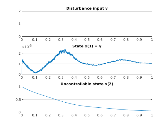
Check optimal L2 with simulation
rho = @(t) [
    min(max(sin(14*t) + randn(size(t)) * rho1_lim(2),rho1_lim(1)),rho1_lim(2))
    min(max(sin(41*t) + randn(size(t)) * rho2_lim(2),rho2_lim(1)),rho2_lim(2))
    ];

% v = @(t) sign(sin(31*t.^2));
v = @(t) ones(size(t));

f_ode = @(t,x) A_fh(rho(t))*x + B_fh(rho(t))*(-K*x + v(t));

[t,x] = ode45(f_ode, [0,1], [0;1]);

y = C*x';

figure

subplot(311), plot(t,v(t)), grid on, title 'Disturbance input v'
subplot(312), plot(t,x(:,1)), grid on, title 'State x(1) = y'
subplot(313), plot(t,x(:,2)), grid on, title 'Uncontrollable state x(2)'

L2_norm = @(t,u) sqrt( trapz(t,u.^2) );

L2_norm_of_v = L2_norm(t,v(t))

L2_norm_of_y = L2_norm(t,y)

Output_gain_for_this_input = L2_norm_of_y / L2_norm_of_v


return
Output:
L2_norm_of_v =

     1


L2_norm_of_y =

    0.0012


Output_gain_for_this_input =

    0.0012
Using the Robust Control Toolbox
Unfortunatelly we do not have this toolbox yet.
d1 = ureal('d1', 0, 'Range', rho_lim(1,:));
d2 = ureal('d2', 0, 'Range', rho_lim(2,:));


A = [
         2*d1 - 3,        0,        0,             0,        0
                0, d1/2 - 1,        0,             0,        0
    d2 - 2*d1 + 2,        0,   d2 - 1,             0,        0
           2 - d2,        0, 4 - 2*d1, 2*d1 + d2 - 5, 2*d1 - 4
    d2 - 2*d1 + 2,        0,        0,             0,   d2 - 1
    ];


B = [
                -1
                 0
     d2 - 2*d1 - 5
     2*d2 - d1 - 2
          - d1 - 2
    ];

C = [ -3    4   -2    2    4 ];

D = 0;

sys_unc = ss(A,B,C,D);
simplify(sys_unc,'full');

figure
bopts = bodeoptions;
bopts.MagUnits = 'abs';
% bodeplot(sys_unc,bopts), grid on;
bodeplot(gridureal(sys_unc,30), bopts), grid on

Nr_samples = 2500;
[peak_gain,freki] = getPeakGain(gridureal(sys_unc,Nr_samples));

[peak_gain,I] = max(peak_gain);

[wcg,wcu] = wcgain(sys_unc)
sys_fdb = ss(A-B*K,B,C,D);
simplify(sys_fdb,'full');

figure
bopts = bodeoptions;
bopts.MagUnits = 'abs';
% bodeplot(sys_unc,bopts), grid on;
bodeplot(gridureal(sys_fdb,30), bopts), grid on

Nr_samples = 2500;
[peak_gain,freki] = getPeakGain(gridureal(sys_fdb,Nr_samples));

[peak_gain,I] = max(peak_gain);

[wcg,wcu] = wcgain(sys_fdb)