Tartalomjegyzék

Van der Pol Oscillator

Teljes Matlab script kiegészítő függvényekkel.

File: vanderpol.m
Directory: 4_gyujtemegy/11_CCS/_1_ccs/ccs_2020/vanderpol
Author: Peter Polcz (ppolcz@gmail.com)

Created on 2020. October 08. (2020b)

Simulate the van der Pol model

fig = figure(1);
delete(fig.Children)

syms t x1 x2 real
x = [x1;x2];

Van der Pol oscillator

The nondimensional input/output equation of the system is:

$\ddot{y} - \mu(1 - y^2) \dot y + y = 0$.

Setting $x_1 = y$ and $x_2 = \dot y$, we obtain the following state-space model:

$\begin{aligned} &\dot{x}_1 = x_2 \\ &\dot{x}_2 = -x_1 + \mu(1 - x_1)^2 x_2 \end{aligned}$

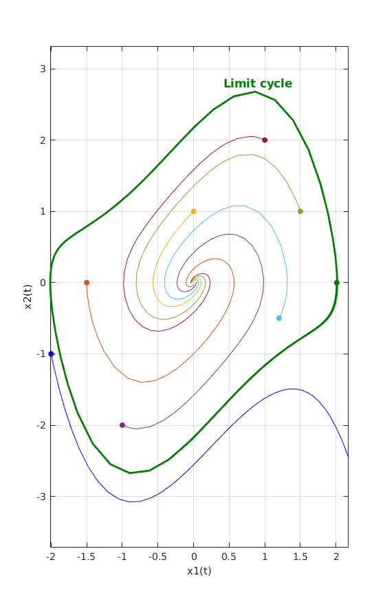
Original van der Pol system, which has globally attractive a limit cycle. Every trajectory will tend to this limit cycle,

vdp_oscillator_sym = [
    x2
    (1 - x1^2)*x2 - x1
    ];
vdp_oscillator_fh = matlabFunction(vdp_oscillator_sym,'vars', {t x});

Time inverted model

If we compute the time inverted model, we obtain a locally asymptotically stable system, for which the domain of attraction is bounded by the original system's limit cycle.

Let $x(t) \leftarrow x(-t)$, then:

$\begin{aligned} &\dot{x}_1 = - x_2 \\ &\dot{x}_2 = x_1 - \mu(1 - x_1)^2 x_2 \end{aligned}$

vdp_inverted_sym = [
    -x2
    -(1 - x1^2)*x2 + x1
    ];
vdp_inverted_fh = matlabFunction(vdp_inverted_sym,'vars', {t x});

Simulate a trajectory of the original van der Pol oscillator, to obtain the limit cycle

simulate(vdp_oscillator_fh,[0 9],[2.01;0],'LineWidth',2,'Color',[0 0.5 0])

Simulate some convergent trajectories of the time-inverted (locally asymptotically stable) van der Pol system

simulate(vdp_inverted_fh,[0 9],[
    0 1.5 1 -1.5 -1  1.2
    1 1   2  0   -2 -0.5 ])

Simulate some diverging trajectories of the time-inverted system

simulate(vdp_inverted_fh,[0 2],[-2;-1],'b')

Visualization

xlabel('x1(t)');
ylabel('x2(t)');

TxT = text(0.9,2.8,'Limit cycle');
TxT.HorizontalAlignment = 'center';
TxT.FontSize = 12;
TxT.FontWeight = 'bold';
TxT.Color = [0 0.5 0];

function simulate(fh,Tspan,ics,varargin)

    figure(1);
    hold on

    for x0 = ics

        [~,x] = ode45(fh,Tspan,x0);

        Pl = plot(x(:,1),x(:,2),varargin{:});
        plot(x(1,1),x(1,2),'.','MarkerSize',20,'Color',Pl.Color)

    end

    grid on
    box on
    axis equal
end

Published with MATLAB® R2020b, and sanitarized by BeautifulSoup (Python script using BSoup is written by Polcz).