Tartalomjegyzék

Inverted pendulum control and reference tracking (servo)

Teljes Matlab script kiegészítő függvényekkel.

file:   ipend2.m
author: Peter Polcz <ppolcz@gmail.com>

Created on 2017.05.02. Tuesday, 22:39:05
Reviewed on 2017. November 22. [servo control]
Reviewed on 2017. November 29. [augmented, corrected, published]

Helper functions: ipend_simulate_Pi.m, ipend_simulate_0.m.

Helper scripts: ipend1_levezetesek.m.

try c = evalin('caller','p100ersist'); catch; c = []; end
persist = pcz_persist(mfilename('fullpath'), c); clear c;
persist.backup();
%clear persist

global PUBLISH
PUBLISH = 1;

open_system ipend2_sim_servo
open_system ipend2_sim_servo_baby

Output:

│   - Persistence for `ipend2` initialized [run ID: 48, 215]Persistence for `2017.11.29. Wednesday, 15:19:19`
│   - Script `ipend2` backuped

Nonlinear model - parameters (A)

No friction

syms t x v phi omega

% model parameters
M = 0.5;
m = 0.2;
l = 1;
g = 9.8;
b = 0;

q = 4*(M+m) - 3*m*cos(phi)^2;

f_sym = [
    v
    (4*m*l*sin(phi)*omega^2 - 1.5*m*g*sin(2*phi) -4*b*v) / q
    omega
    3*(-m*l*sin(2*phi)*omega^2 / 2 + (M+m)*g*sin(phi) + b*cos(phi)*v) / (l*q)
    ];

g_sym = [
    0
    4*l
    0
    -3*cos(phi)
    ] / (l*q);

f_ode = matlabFunction(f_sym, 'vars', {t , [ x ; v ; phi ; omega ]});
g_ode = matlabFunction(g_sym, 'vars', {t , [ x ; v ; phi ; omega ]});

Linearized model around the unstable equilibrium point

% model parameters
M = 0.5;
m = 0.2;
l = 1;
g = 9.8;
b = 0;

A = [
    0                     1                             0  0
    0      -(4*b)/(4*M + m)            -(3*g*m)/(4*M + m)  0
    0                     0                             0  1
    0   (3*b)/(l*(4*M + m))   (3*g*(M + m))/(l*(4*M + m))  0
    ];

B = [
    0
    4/(m+4*M)
    0
    -3/(m+4*M)/l
    ];

C = [
    1 0 0 0
    0 0 1 0
    ];

D = [ 0 ; 0 ];

sys = ss(A,B,C,D);

K = place(A,B,-4:-1);
pcz_num2str(K)

K = lqr(A,B,eye(4),1);
pcz_num2str(K)

L = place(A',C',-4:0.1:-3.7)'
pcz_num2str(L)

Output:

[ -1.7959 , -3.7415 , -34.9212 , -12.322 ]
[ -1 , -2.2428 , -26.6075 , -9.3028 ]
L =
    7.6382    0.0811
   14.5773   -2.3605
    0.0761    7.7618
    0.2935   24.4073
[ 7.6382 , 0.0811 ; 14.5773 , -2.3605 ; 0.0761 , 7.7618 ; 0.2935 , 24.4073 ]

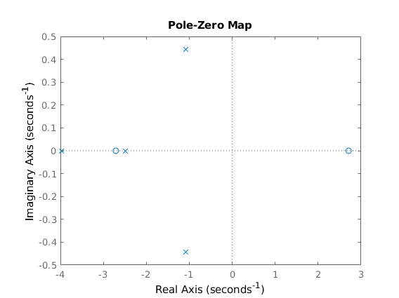
Transfer function of the closed loop system

Ac = [ A-B*K B*K ; zeros(4,4) A-L*C ];
Bc = [ B ; zeros(4,1) ];
Cc = [ 1 0 0 0 -1 0 0 0 ];
Dc = 0;

cls = ss(Ac,Bc,Cc,Dc);
Ge = minreal(tf(cls))
pzmap(Ge)

Gi = pidtune(Ge,'I')

G_all = minreal(Ge*Gi / (1 + Ge*Gi));

Output:

Ge =

         1.818 s^2 + 3.23e-15 s - 13.36
  ---------------------------------------------
  s^4 + 8.608 s^3 + 25.11 s^2 + 29.97 s + 13.36

Continuous-time transfer function.


Gi =

        1
  Ki * ---
        s

  with Ki = -0.241

Continuous-time I-only controller.

Linear-Quadratic-Integral control: lqi

C = [
    1 0 0 0
    ];

D = [ 0 ];

sys = ss(A,B,C,D);

K = lqr([A zeros(4,1) ; -C 0], [B ; 0], eye(5), 1)

K_lqi = lqi(sys, 1*eye(5),1);
K = K_lqi(:,1:4);
Ki = -K_lqi(end);

set_param('ipend2_sim_servo/K_lqi','Gain',pcz_num2str(-K_lqi))
set_param('ipend2_sim_servo_baby/K_x','Gain',pcz_num2str(K))
set_param('ipend2_sim_servo_baby/K_I','Gain',pcz_num2str(Ki))

Output:

K =
   -2.9469   -3.8422  -33.7982  -11.9483    1.0000

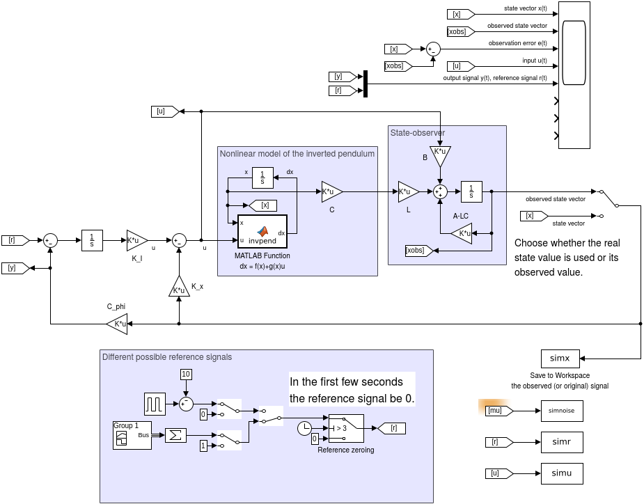
Simulate simulink results (baby model)

Simulink model: ipend2_sim_servo_baby.slx

open_system ipend2_sim_servo_baby
print -dpng fig/ipend2_sim_servo_baby.png -sipend2_sim_servo_baby

Simulate

sim ipend2_sim_servo_baby

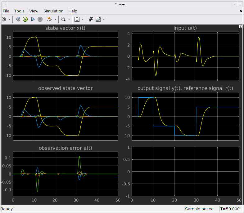
Visualize external control force

t = simx.Time;
x = simx.Data;
u = simu.Data;
r = simr.Data;
ipend_simulate_0(t,x,u,r)

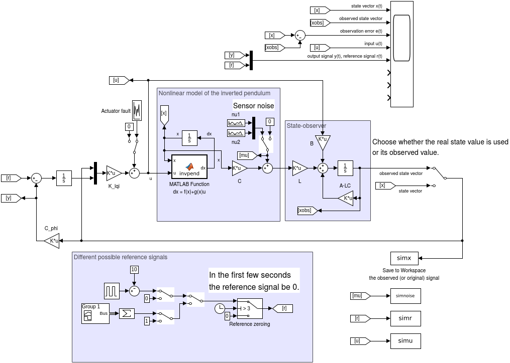
Simulate simulink results (expert model)

Simulink model: ipend2_sim_servo.slx

open_system ipend2_sim_servo
print -dpng fig/ipend2_sim_servo.png -sipend2_sim_servo

Simulate

sim ipend2_sim_servo

Visualize external control force

t = simx.Time;
x = simx.Data;
u = simu.Data;
r = simr.Data;
ipend_simulate_0(t,x,u,r)

Published with MATLAB® R2017b, and sanitarized by BeautifulSoup (Python script using BSoup is written by Polcz).