Tartalomjegyzék
\[ \newenvironment{dcases}{\left\{\begin{array}{ll}}{\end{array}\right.} \]Inverted pendulum control and analysis
Teljes Matlab script kiegészítő függvényekkel.
file:   ipend.m
author: Peter Polcz <ppolcz@gmail.com>
Created on 2017.03.27. Monday, 17:42:37
Reviewed on 2017. October 30. [Published]
Reviewed on 2017. November 08. [Corrected and published]
try c = evalin('caller','persist'); catch; c = []; end
persist = pcz_persist(mfilename('fullpath'), c); clear c;
persist.backup();
%clear persist

global PUBLISH
PUBLISH = 1;
Output:
│   - Persistence for `ipend1` reused (inherited) [run ID: 48, 036]Persistence for `2017.11.09. Thursday, 11:25:23`
│   - Script `ipend1` backuped
A. Linearize around the stable equilibrium point
State space model
% model parameters
M = 0.5;
m = 0.2;
l = 1;
g = 9.8;
b = 0;

A = [
    0                     1                             0  0
    0      -(4*b)/(4*M + m)            -(3*g*m)/(4*M + m)  0
    0                     0                             0  1
    0  -(3*b)/(l*(4*M + m))  -(3*g*(M + m))/(l*(4*M + m))  0
    ];

B = [
    0
    4/(m+4*M)
    0
    3/(m+4*M)/l
    ];

C = [
    1 0 0 0
    0 0 1 0
    ];

D = [ 0 ; 0 ];
1. determine the transfer function of the system
sys = ss(A,B,C,D);
H = tf(sys);

H_r = H(1)
H_phi = H(2)
Output:
H_r =

  1.818 s^2 + 13.36
  -----------------
   s^4 + 9.355 s^2

Continuous-time transfer function.


H_phi =

     1.364
  -----------
  s^2 + 9.355

Continuous-time transfer function.
2. determine the impulse response of the system
T = 5;
[y,t] = impulse(H,T);
ipend_simulate_Pi(t,y)
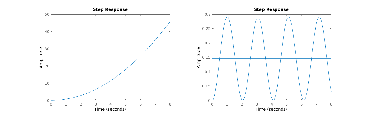
3. determine the step response and the DC gain of the system
T = 8;

figure('Position', [ 226 318 1276 392 ], 'Color', [1 1 1])

subplot(121)
step(H_r,T)

subplot(122)
step(H_phi,T), hold on

DC_gain = dcgain(H_phi);
plot([0 T],[1 1]*DC_gain)
Simulate
[y,t] = step(H,T);
ipend_simulate_Pi(t,y)
4. determine the poles of the system
Is the system stable, exponentially stable or unstable
eig(A)
Output:
ans =
   0.0000 + 0.0000i
   0.0000 + 0.0000i
   0.0000 + 3.0585i
   0.0000 - 3.0585i
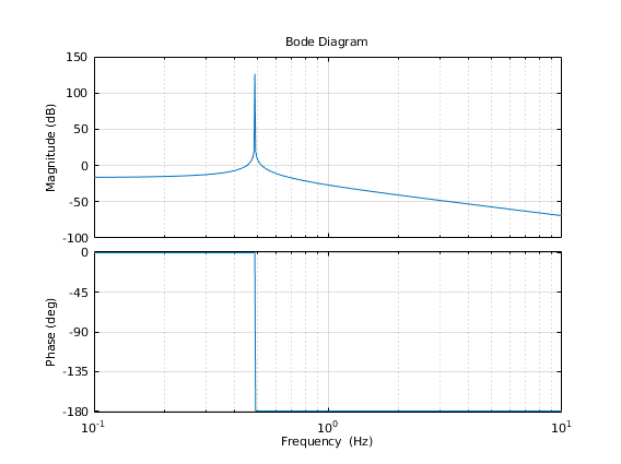
5. determine the Bode plot of the transfer function
Plot only for the transfer function from F to omega. The frequency unit set to be in Hz. Determine the own (or resonance) frequency (f_r) of the system.
figure
bopts = bodeoptions;
bopts.FreqUnits = 'Hz';
% bopts.FreqScale = 'linear';
% bopts.MagUnits = 'abs';
bodeplot(H_phi, bopts), grid on

[gpeak,fpeak] = getPeakGain(H_phi);
fr = fpeak / (2*pi)
Output:
fr =
    0.4868
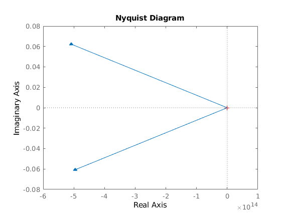
6. Nyquist plot
figure(6), nyquist(H_phi)
7. (a) Simulation using lsim - resonance frequency
T = 20;
Ts = 0.01;
t = 0:Ts:T;

f = fr;
Amp = 1;
u = Amp*sin(2*pi*f*t);
y = lsim(H,u,t);
ipend_simulate_Pi(t,y,u);

% After a while we shall notice, that the system's motion is quite
% unusual, why?
7. (b) Simulation using lsim - high frequency, large amplitude
T = 10;
Ts = 0.01;
t = 0:Ts:T;

f = 4;
Amp = 20;
u = Amp*sin(2*pi*f*t)-0.1;
y = lsim(H,u,t);
ipend_simulate_Pi(t,y,u);
7. (c) Simulation using lsim - low frequency
T = 20;
Ts = 0.01;
t = 0:Ts:T;

f = 0.1;
Amp = 1;
u = Amp*sin(2*pi*f*t + pi/2);
y = lsim(H,u,t);
ipend_simulate_Pi(t,y,u);
8. Simulation using ode45
x0 = [0 0 pi/6 0]';
u = 0;
T = 5;
[t,x] = ode45(@(t,x) A*x + B*u, [0 T], x0);
ipend_simulate_Pi(t,x)
9. Controllability
C4 = [ B A*B A*A*B A*A*A*B ]
C4_ = ctrb(A,B);
rank(C4)
Output:
C4 =
         0    1.8182         0   -3.6446
    1.8182         0   -3.6446         0
         0    1.3636         0  -12.7562
    1.3636         0  -12.7562         0
ans =
     4
10. Observability
C = [
    1 0 0 0
    0 0 1 0
    ];

O4 = obsv(A,C)
O4_ = ctrb(A',C')'

rank(O4)

% Measure only phi
C = [ 0 0 1 0 ];

O4 = obsv(A,C);
S = [ orth(O4) null(O4) ];
T = inv(S);

A_ = T*A/T
B_ = T*B
C_ = C/T
Output:
O4 =
    1.0000         0         0         0
         0         0    1.0000         0
         0    1.0000         0         0
         0         0         0    1.0000
         0         0   -2.6727         0
         0         0   -9.3545         0
         0         0         0   -2.6727
         0         0         0   -9.3545
O4_ =
    1.0000         0         0         0
         0         0    1.0000         0
         0    1.0000         0         0
         0         0         0    1.0000
         0         0   -2.6727         0
         0         0   -9.3545         0
         0         0         0   -2.6727
         0         0         0   -9.3545
ans =
     4
A_ =
         0   -1.0000         0         0
    9.3545         0         0         0
         0         0         0   -1.0000
    3.6519         0         0         0
B_ =
         0
    1.3714
         0
    1.9640
C_ =
   -0.9943         0         0         0
B. Nonlinear model. No friction
Input affine model
$$\dot x = f(x) + g(x) u$$
syms t x v phi omega

% model parameters
M = 0.5;
m = 0.2;
l = 1;
g = 9.8;
b = 0;

q = 4*(M+m) - 3*m*cos(phi)^2;

f_sym = [
    v
    (4*m*l*sin(phi)*omega^2 - 1.5*m*g*sin(2*phi) -4*b*v) / q
    omega
    3*(-m*l*sin(2*phi)*omega^2 / 2 + (M+m)*g*sin(phi) + b*cos(phi)*v) / (l*q)
    ];

g_sym = [
    0
    4*l
    0
    -3*cos(phi)
    ] / (l*q);

f_ode = matlabFunction(f_sym, 'vars', {t , [ x ; v ; phi ; omega ]});
g_ode = matlabFunction(g_sym, 'vars', {t , [ x ; v ; phi ; omega ]});
11. Simulation with no input
[tt,xx] = ode45(f_ode, [0,10], [0 0 0.1 0]');
ipend_simulate_0(tt,xx)

[tt,xx] = ode45(f_ode, [0,10], [0 0 0.1 2]');
ipend_simulate_0(tt,xx)
11. Simulation with large amplitude high frequency sinusoidal signal
Ampl = 20;
f = 4;
u = @(t) Ampl*sin(2*pi*f*t);
[tt,xx] = ode45(@(t,x) f_ode(t,x) + g_ode(t,x)*u(t), [0,5], [0 0 pi 0]');
ipend_simulate_0(tt,xx,u)
11. Simulation with small amplitude own frequency sinusoidal signal
Ampl = 1;
f = fr;
u = @(t) Ampl*sin(2*pi*f*t);
[tt,xx] = ode45(@(t,x) f_ode(t,x) + g_ode(t,x)*u(t), [0,30], [0 0 pi 0]');
ipend_simulate_0(tt,xx,u)
11. Simulation with small amplitude low frequency sinusoidal signal
Ampl = 1;
f = 0.1;
u = @(t) Ampl*sin(2*pi*f*t + pi/2);
[tt,xx] = ode45(@(t,x) f_ode(t,x) + g_ode(t,x)*u(t), [0,30], [0 0 pi 0]');
ipend_simulate_0(tt,xx,u)
C. Nonlinear model. With friction
Input affine model
$$\dot x = f(x) + g(x) u$$
syms t x v phi omega

% model parameters
M = 0.5;
m = 0.2;
l = 1;
g = 9.8;
b = 10;

q = 4*(M+m) - 3*m*cos(phi)^2;

f_sym = [
    v
    (4*m*l*sin(phi)*omega^2 - 1.5*m*g*sin(2*phi) -4*b*v) / q
    omega
    3*(-m*l*sin(2*phi)*omega^2 / 2 + (M+m)*g*sin(phi) + b*cos(phi)*v) / (l*q)
    ];

g_sym = [
    0
    4*l
    0
    -3*cos(phi)
    ] / (l*q);

f_ode = matlabFunction(f_sym, 'vars', {t , [ x ; v ; phi ; omega ]});
11. Simulation
[t,x] = ode45(f_ode, [0,10], [0 0 pi/12 2]');
ipend_simulate_0(t,x)
D. Linear model with friction PID controller
State space model
model parameters
M = 0.5;
m = 0.2;
l = 1;
g = 9.8;
b = 0;

A = [
    0                     1                             0  0
    0      -(4*b)/(4*M + m)            -(3*g*m)/(4*M + m)  0
    0                     0                             0  1
    0  -(3*b)/(l*(4*M + m))  -(3*g*(M + m))/(l*(4*M + m))  0
    ];

B = [
    0
    4/(m+4*M)
    0
    3/(m+4*M)/l
    ];

C = [
    1 0 0 0
    0 0 1 0
    ];

D = [ 0 ; 0 ];
Transfer function of the system
sys = ss(A,B,C,D);
H = tf(sys);
H_r = H(1);
H_phi = H(2);
PID for the non-inverted pendulum, reference tracking
Only if $b \not= 0$!
open_system ipend_PID_demo
print -dpng fig/ipend_PID.png -sipend_PID_demo
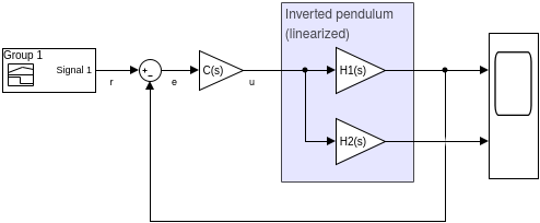
C_r = pidtune(H_r,'pid');
% pidTuner(H_r,C_r)
At home: derive the resulting transfer function
Control_Loop = [
    C_r*H_r / (1 + C_r*H_r)
    C_r*H_phi / (1 + C_r*H_r)
    ];

T = 20;
t = linspace(0,T,T/0.1);
u = t*0 + 5;
y = lsim(Control_Loop,u,t);
ipend_simulate_Pi(t,y)