Tartalomjegyzék
\[ \newenvironment{dcases}{\left\{\begin{array}{ll}}{\end{array}\right.} \]Geometrical meaning of Lie derivative
Teljes Matlab script kiegészítő függvényekkel.
File: lie_geometrical_meaning.m
Directory: 4_gyujtemegy/11_CCS/_2_nonlin-pannon/2018
Author: Peter Polcz (ppolcz@gmail.com)
Created on 2018. July 29.
Requirements
vekanal_subsmesh.m, vekanal_quiver_sym.m and pcz_arrow.m
syms t x1 x2 real

x = [ x1 ; x2 ];

Lie = @(f,h) jacobian(h,x) * f;

f = [
    x2 + 0.4*x2*x1
    -x1-x2 + 0.3*x1^2
    ];

h = sin(x1+x2^2)^2 + x2^2;

Lfh = Lie(f,h);
Lfh_fh = matlabFunction(Lfh,'vars',{x'});
$$L_f h(x) = 2\,\cos\left({x_{2}}^2+x_{1}\right)\,\sin\left({x_{2}}^2+x_{1}\right) \,\left(x_{2}+\frac{2\,x_{1}\,x_{2}}{5}\right)-\left(2\,x_{2}+4\,x_{2} \,\cos\left({x_{2}}^2+x_{1}\right)\,\sin\left({x_{2}}^2+x_{1}\right)\right) \,\left(-\frac{3\,{x_{1}}^2}{10}+x_{1}+x_{2}\right)$$
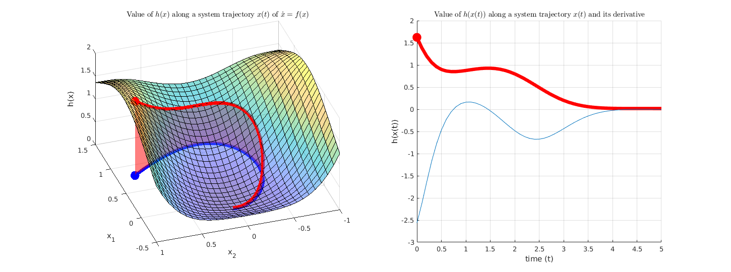
The blue line is a system trajectory of $\dot x = f(x)$ with the initial condition illustrated by the blue dot. The red line highlights the value of function $h(x)$ along the trajectory $x(t)$. In this way $h(x(t))$ can be considered as a scalar function of $t$. Its time derivative can be computed by the chain rule: $\frac{\mathrm{d}}{\mathrm{d} t} h(x(t)) = \frac{\partial h}{\partial x} \cdot \dot x = \frac{\partial h}{\partial x} f(x)$.
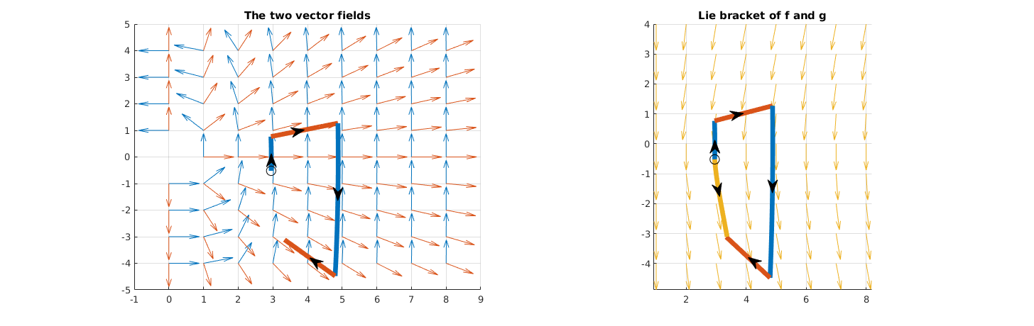
Geometrical meaning of the Lie bracket
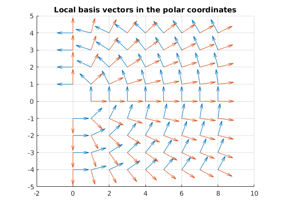
Local basis vectors in polar coordinates as two vector fields
syms x y real

Z = [x;y];

f_sym = [
    -y
    x
    ];

g_sym = [
    x
    y
    ] / sqrt(x^2 + y^2);

figure, hold on, grid on
Q1 = vekanal_quiver_sym(f_sym, Z, {0,8,9}, {-4,4,9}, 0.7);
Q2 = vekanal_quiver_sym(g_sym, Z, {0,8,9}, {-4,4,9}, 0.7);
title 'Local basis vectors in the polar coordinates'
Output:
br_fg =
 0
 0
Path 1 starting from from (2.95,-0.52):
 -   0.4 seconds along the flow of f(x,y)
 -   1 seconds along the flow of g(x,y)
 -   -0.4 seconds along the flow of f(x,y) (i.e. moving backwards)
 -   -1 seconds along the flow of g(x,y) (i.e. moving backwards)

Path 2 starting from from (1.88,-0.68):
 -   0.8 seconds along the flow of f(x,y)
 -   3 seconds along the flow of g(x,y)
 -   -0.8 seconds along the flow of f(x,y) (i.e. moving backwards)
 -   -3 seconds along the flow of g(x,y) (i.e. moving backwards)

Path 3 starting from from (0.77,-0.64):
 -   1.4 seconds along the flow of f(x,y)
 -   5 seconds along the flow of g(x,y)
 -   -1.4 seconds along the flow of f(x,y) (i.e. moving backwards)
 -   -5 seconds along the flow of g(x,y) (i.e. moving backwards)
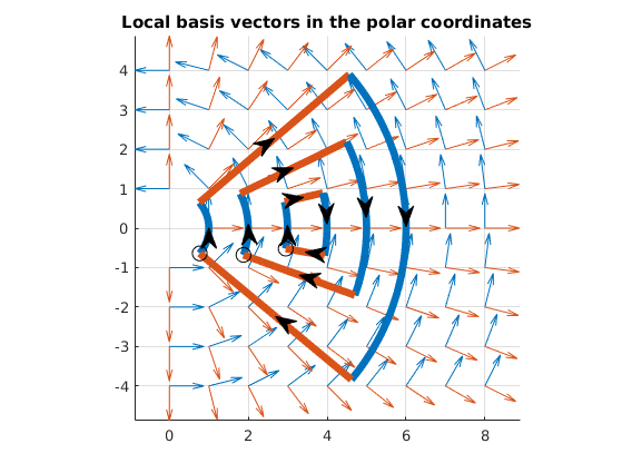
A walk along the flow of f and g and then backwards is closed.
What if the Lie bracket is non-zero
syms x y real

Z = [x;y];

f_sym = [
    -y
    x^3
    ];

g_sym = [
    x
    y
    ] / sqrt(x^2 + y^2);

br_fg = simplify(jacobian(g_sym,Z)*f_sym - jacobian(f_sym,Z)*g_sym);
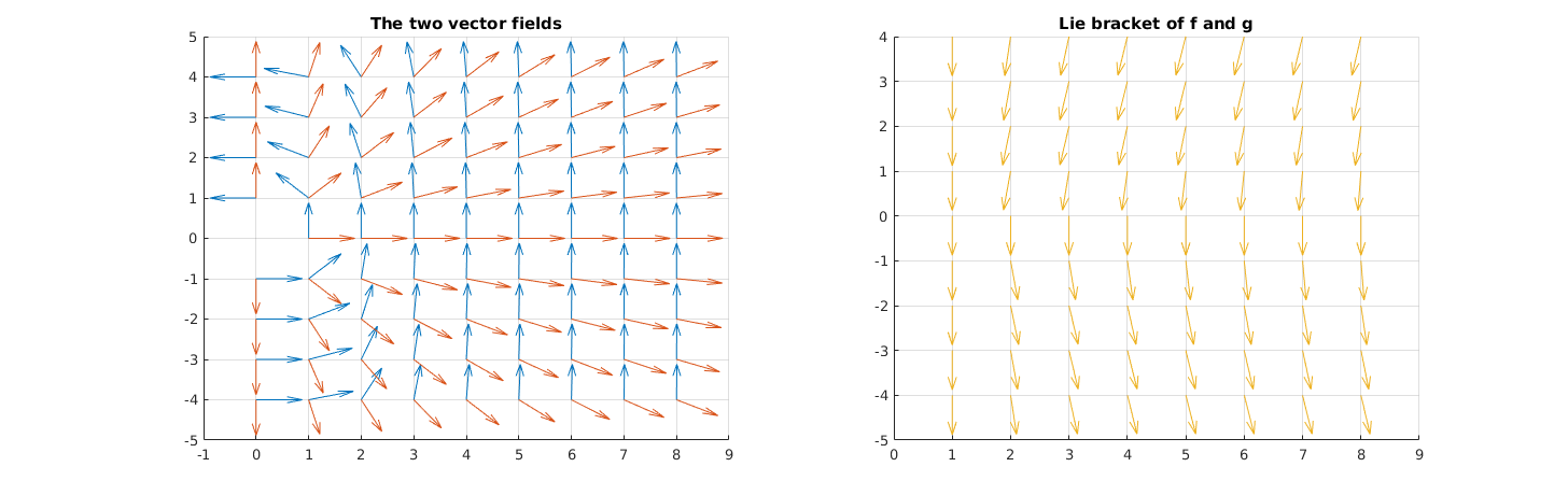
The walk along the flow of f and g is not closed
Output:
Path 1 starting from from (2.95,-0.52):
 -   0.05 seconds along the flow of f(x,y)
 -   2 seconds along the flow of g(x,y)
 -   -0.05 seconds along the flow of f(x,y) (i.e. moving backwards)
 -   -2 seconds along the flow of g(x,y) (i.e. moving backwards)